Page 286 - Applied statistics and probability for engineers

264 Chapter 7/Point Estimation of Parameters and Sampling Distributions

When the derivatives are equated to zero, we obtain the equations that must be solved to ind the maximum likelihood
estimators of r and λ:
ˆ
λ = ˆ r
x
n Γ′ r ( ) ˆ
ˆ
)
n ln( λ + ∑ ln( x i = n
)
i=1 Γ r ( ) ˆ
There is no closed form solution to these equations.
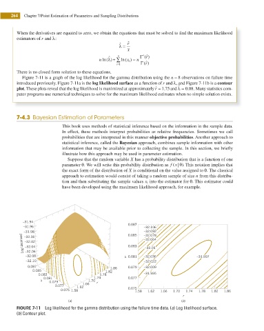
Figure 7-11 is a graph of the log likelihood for the gamma distribution using the n = 8 observations on failure time
introduced previously. Figure 7-11a is the log likelihood surface as a function of r and λ, and Figure 7-11b is a contour
ˆ
plot. These plots reveal that the log likelihood is maximized at approximately ˆ r = .1 75 and λ = .0 08. Many statistics com-
puter programs use numerical techniques to solve for the maximum likelihood estimates when no simple solution exists.

7-4.3 Bayesian Estimation of Parameters

This book uses methods of statistical inference based on the information in the sample data.
In effect, these methods interpret probabilities as relative frequencies. Sometimes we call
probabilities that are interpreted in this manner objective probabilities. Another approach to
statistical inference, called the Bayesian approach, combines sample information with other
information that may be available prior to collecting the sample. In this section, we briel y
illustrate how this approach may be used in parameter estimation.
Suppose that the random variable X has a probability distribution that is a function of one
parameter θ. We will write this probability distribution as f x( | θ ). This notation implies that
the exact form of the distribution of X is conditional on the value assigned to θ. The classical
approach to estimation would consist of taking a random sample of size n from this distribu-
tion and then substituting the sample values x i into the estimator for θ. This estimator could
have been developed using the maximum likelihood approach, for example.

–31.94
–31.96 0.087 –32.106
–31.98 0.085 –32.092
–32.078
Log likelihood –32.02 0.083 –32.064
–32.00
–32.04
–32.05
–32.06
–32.08 l 0.081 –32.036 –31.997
–32.10 –32.022
0.087 1.86 0.079 –32.009
0.085 1.82
0.083 1.78 –31.995
0.081 1.74 0.077
l 0.079 1.70 r
0.077 1.62 1.66
0.075 1.58 0.075 1.58 1.62 1.66 1.70 1.74 1.78 1.82 1.86
r
(a) (b)
FIGURE 7-11 Log likelihood for the gamma distribution using the failure time data. (a) Log likelihood surface.
(b) Contour plot.