Page 288 - Applied statistics and probability for engineers

266 Chapter 7/Point Estimation of Parameters and Sampling Distributions

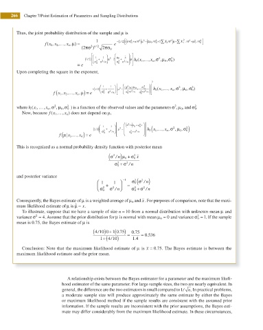
Thus, the joint probability distribution of the sample and μ is

2
2
2
2
/
μ
/ ) μ+ ∑ x i
0
f x , x , … , x , ) = 1 e −( / 1 2) ( ⎢ ⎡ ⎣ 1 σ +/ 2 0 n ) μ − μ/σ 2 2 ( 2 0 /σ + ∑ x i σ 2 2 / σ +μ 0 / σ 2 0 ⎤ ⎦ ⎥
2
n
( 1
(2πσ 2 ) n/ 2 2πσ 0
⎡ ⎛ ⎞ ⎛ − ⎞ ⎤
μ
− (1 2 / ) ⎜ ⎢ ⎢ ⎜ 1 + 1 ⎟ μ −2 ⎜ μ 0 + x ⎟ ⎥ n x σ , 2 ,μ È , 2 0 )
2
⎟ ⎥ h x …,( ,
⎜ ⎝ ⎢ σ 2 σ 2 n / ⎠ ⎟ ⎜ ⎜ σ 2 σ 2 n / ⎟ ⎥ 1 1 μ 0
= e ⎣ 0 ⎝ 0 ⎠ ⎦
Upon completing the square in the exponent,
2
⎡
⎛ 1 + 1 ⎞ ⎟ μ − ⎛ σ ( 2 n / ) μ 0 + x σ 2 0 ⎞ ⎤ 2 h x , …, x , σ , μ 0 , σ 0 )

(
2
⎢
⎟ ⎥
2
2 ⎜
( −
/ 1 2)⎜
1 (
2
2
…
f x , x , , x , μ) = e ⎜ ⎝ σ 2 0 σ 2 / n⎠ ⎟ ⎢ ⎣ ⎢ ⎜ ⎝ σ 2 ++σ /n σ 2 0 +σ /n ⎟ ⎥ 1 n
⎠ ⎦ ⎥
0
n
2
where h x( , 1 … , x n , È μ σ , 2 0 ) is a function of the observed values and the parameters σ , μ 0 , and σ 0 .
2
2
2
,
i
0
Now, because f x( , ... , x n ) does not depend on μ,
1
⎡ ⎛ σ ( 2 x ⎞ ⎤
⎛ 1 1 ⎞ ⎢ ⎜ /n) μ + σ 2 0 ⎟ ⎥ σ )
0
2
⎢
2
− / (1 2 )⎜ ⎜ 2 + 2 ⎟ μ − ⎜ 2 ⎟ ⎥ h x , …, x , σ , μ 0 , 2 0
3
⎟
( 1
n
f μ| ( x , , x n) = e ⎝ σ 0 σ /n ⎠ ⎢ ⎢ ⎣ ⎜ ⎝ σ 2 + σ /n ⎟ ⎥ ⎥
+
…
0
⎠ ⎦
1
This is recognized as a normal probability density function with posterior mean
σ ( 2 / n ) μ + σ 0 x
2
0
2
2
σ + σ / n
0
and posterior variance
2
⎛ 1 1 ⎞ − 1 0 σ σ ( 2 / ) n
⎜ ⎝ 0 σ 2 + σ / n ⎟ ⎠ = 2 0 σ + σ / n
2
2
Consequently, the Bayes estimate of μ is a weighted average of μ 0 and x. For purposes of comparison, note that the maxi-
mum likelihood estimate of μ is ˆ μ = x.
To illustrate, suppose that we have a sample of size n = 10 from a normal distribution with unknown mean μ and
variance σ = 4. Assume that the prior distribution for μ is normal with mean μ 0 = 0 and variance σ = 1. If the sample
2
2
0
mean is 0.75, the Bayes estimate of μ is
)
+ (
4 10 0 1 0 75) 0 75
/ (
.
.
0 536
1+( 4 10) = 1 4 . = .
/
Conclusion: Note that the maximum likelihood estimate of μ is x = .75. The Bayes estimate is between the
0
maximum likelihood estimate and the prior mean.
A relationship exists between the Bayes estimator for a parameter and the maximum likeli-
hood estimator of the same parameter. For large sample sizes, the two are nearly equivalent. In
general, the difference are the two estimators is small compared to 1/ n. In practical problems,
a moderate sample size will produce approximately the same estimate by either the Bayes
or maximum likelihood method if the sample results are consistent with the assumed prior
information. If the sample results are inconsistent with the prior assumptions, the Bayes esti-
mate may differ considerably from the maximum likelihood estimate. In these circumstances,