Page 285 - Applied statistics and probability for engineers

Section 7-4/Methods of Point Estimation 263

Complications in Using Maximum Likelihood Estimation
Although the method of maximum likelihood is an excellent technique, sometimes complica-
tions arise in its use. For example, it is not always easy to maximize the likelihood function
because the equation(s) obtained from dL( )θ / dθ = 0 may be difi cult to solve. Furthermore, it
may not always be possible to use calculus methods directly to determine the maximum of L( )θ .
These points are illustrated in the following two examples.

Example 7-15 Uniform Distribution MLE Let X be uniformly distributed on the interval 0 to a. Because the
density function is f x) = 1 for 0 ≤ x ≤ a and zero otherwise, the likelihood function of a random
(
a /
sample of size n is
n 1 1
L a ( ) = Π =
for i=1 a a n
0 ≤ x 1 ≤ a, 0 ≤ x 2 ≤ a, …, 0 ≤ x n ≤ a
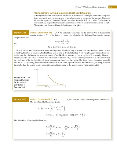
Note that the slope of this function is not zero anywhere. That is, as long as max( )x i ≤ a, the likelihood is 1/ a , which
n
is positive, but when a < max( ), the likelihood goes to zero as illustrated in Fig. 7-10. Therefore, calculus methods can-
x i
not be used directly because the maximum value of the likelihood function occurs at a point of discontinuity. However,
− n n+1 − n
because d / da a ( ) = − n/ a is less than zero for all values of a > 0, a is a decreasing function of a. This implies that

the maximum of the likelihood function L a( ) occurs at the lower boundary point. The igure clearly shows that we could
maximize L a( ) by setting ˆ a equal to the smallest value that it could logically take on, which is max( )x i . Clearly, a cannot
be smaller than the largest sample observation, so setting ˆ a equal to the largest sample value is reasonable.
L(a)

FIGURE 7-10 The
likelihood function
for the uniform
distribution in
Example 7-15. 0 Max (x ) a
i

Example 7-16 Gamma Distribution MLE Let X X 2 ,… , X n be a random sample from the gamma distribution.
1 ,
The log of the likelihood function is
⎛ n r r −1 e −λx i ⎞
ln (r, λ) = ln Π λ x i ⎟
L
⎜
⎝ = i 1 Γ( ) r ⎠
n n
)
= nr ln( ) ( −1) ∑ ln ( ) − ln [ ( ]− λ ∑ x i
n
λ + r
Γ r)
x i
= i 1 = i 1
The derivatives of the log likelihood are
(
∂ ln L r, λ) = ln( ) n ( − n Γ′ r ( )
λ + ∑ ln x i )
n
∂r = i 1 Γ r ( )
∂ ln L r, ( λ) = nr n
∂λ λ − ∑ x i
= i 1