Page 310 - Applied statistics and probability for engineers

288 Chapter 8/Statistical intervals for a single sample

f(x)

k = 2

k = 5
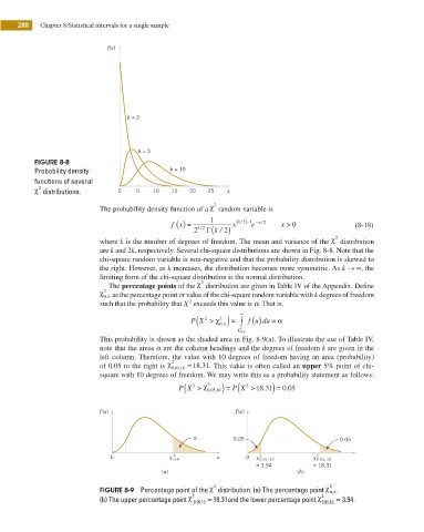
FIGURE 8-8
Probability density k = 10
functions of several
2
χ distributions. 0 5 10 15 20 25 x
χ
2
The probability density function of a random variable is
1
f x ( ) = k/ 2 Γ( x k/ ( 2 )−1 e − x/ 2 x > 0 (8-18)
2 k / ) 2
χ
2
where k is the number of degrees of freedom. The mean and variance of the distribution
are k and 2k, respectively. Several chi-square distributions are shown in Fig. 8-8. Note that the
chi-square random variable is non-negative and that the probability distribution is skewed to
the right. However, as k increases, the distribution becomes more symmetric. As k → ∞ , the
limiting form of the chi-square distribution is the normal distribution.
χ
2
The percentage points of the distribution are given in Table IV of the Appendix. Deine
χ α,k as the percentage point or value of the chi-square random variable with k degrees of freedom
2
2
such that the probability that X exceeds this value is a. That is,
(
( )
P X > χ ) = ∞ ∫ f u du = α
2
2
α
,k
χ 2 α ,k
This probability is shown as the shaded area in Fig. 8-9(a). To illustrate the use of Table IV,
note that the areas α are the column headings and the degrees of freedom k are given in the
left column. Therefore, the value with 10 degrees of freedom having an area (probability)
2
of 0.05 to the right is χ . 0 05 10 = 18 .31 . This value is often called an upper 5% point of chi-
,
square with 10 degrees of freedom. We may write this as a probability statement as follows:
(
P X > χ 2 0 05 ,10) = ( 2 . 0 05
P X >18 31) = .
2
.
f (x) f (x)
0.05 0.05
0 x 0 x 2 0.95, 10 x 2 0.05, 10
= 3.94 = 18.31
(a) (b)

χ
χ
2
2
FIGURE 8-9 Percentage point of the distribution. (a) The percentage point α,k.
(b) The upper percentage point χ 2 0.05,10 = 18.31 and the lower percentage point χ 2 0.95,10 = 3.94.