Page 306 - Applied statistics and probability for engineers

284 Chapter 8/Statistical intervals for a single sample

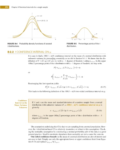
k = 10

k = ` [N (0, 1)]

k = 1

0 x 0 t

FIGURE 8-4 Probability density functions of several FIGURE 8-5 Percentage points of the t
t distributions. distribution.

8-2.2 t CONFIDENCE INTERVAL ON μ
It is easy to ind a 100(1 – α)% conidence interval on the mean of a normal distribution with
unknown variance by proceeding essentially as we did in Section 8-1.1. We know that the dis-
tribution of T = ( X −μ) ( S n) is t with n – 1 degrees of freedom. Letting t / ,nα 2 −1 be the upper
100α / 2 percentage point of the t distribution with n – 1 degrees of freedom, we may write
P − ( t / ,n Ð T≤ t / ,n ) = − α
1
−1
α 2
−1
α 2
or
⎛ X − μ ⎞
⎜ t / ,n Ð t / ,n ⎟ = − α
1
P − α 2 −1 S n ≤ α 2 −1 ⎠
⎝
Rearranging this last equation yields
− (
+
n
1
P X t / ,nα 2 −1 S n Ð μ ≤ X t / ,nα 2 −1 S ) = − α (8-15)
This leads to the following deinition of the 100(1 – α)% two-sided conidence interval on μ.

Conidence
Interval on the If x and s are the mean and standard deviation of a random sample from a normal
Mean, Variance distribution with unknown variance σ , a 100(1 – `)% conidence interval on l is
2
Unknown given by
x − t / ,nα 2 −1 s n Ð μ ≤ x+ t / ,nα 2 −1 s n (8-16)
−1 is the upper 100α 2 percentage point of the t distribution with n – 1
where t / ,nα 2
degrees of freedom.

The assumption underlying this CI is that we are sampling from a normal population. How-
ever, the t distribution-based CI is relatively insensitive or robust to this assumption. Check-
ing the normality assumption by constructing a normal probability plot of the data is a good
general practice. Small to moderate departures from normality are not a cause for concern.
One-sided conidence bounds on the mean of a normal distribution are also of interest and
are easy to ind. Simply use only the appropriate lower or upper conidence limit from Equa-
−1 by
tion 8-16 and replace t / ,nα 2 t ,nα − . 1