Page 301 - Applied statistics and probability for engineers

Section 8-1/Conidence Interval on the Mean of a Normal Distribution, Variance Known 279

8-1.5 LARGE-SAMPLE CONFIDENCE INTERVAL FOR μ
We have assumed that the population distribution is normal with unknown mean and known
standard deviation σ. We now present a large-sample CI for μ that does not require these
assumptions. Let X , X , …, X be a random sample from a population with unknown mean
n
2
1
μ and variance σ . Now if the sample size n is large, the central limit theorem implies
2
2
that X has approximately a normal distribution with mean μ and variance σ /n. Therefore,
Z = ( X − μ) ( σ / n) has approximately a standard normal distribution. This ratio could be
used as a pivotal quantity and manipulated as in Section 8-1.1 to produce an approximate CI
for μ. However, the standard deviation σ is unknown. It turns out that when n is large, replac-
ing σ by the sample standard deviation S has little effect on the distribution of Z. This leads to
the following useful result.
Large-Sample
Coni dence Interval When n is large, the quantity
on the Mean X − μ
S / n
has an approximate standard normal distribution. Consequently,
x − z / 2 s Ð μ ≤ x + z / 2 s (8-11)
α
α
n n

is a large-sample coni dence interval for μ, with conidence level of approximately
100(1 – α)%.

Equation 8-11 holds regardless of the shape of the population distribution. Generally, n should
be at least 40 to use this result reliably. The central limit theorem generally holds for n ≥ 30,
but the larger sample size is recommended here because replacing s with S in Z results in
additional variability.

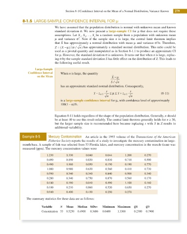
Example 8-5 Mercury Contamination An article in the 1993 volume of the Transactions of the American
Fisheries Society reports the results of a study to investigate the mercury contamination in large-
mouth bass. A sample of ish was selected from 53 Florida lakes, and mercury concentration in the muscle tissue was

measured (ppm). The mercury concentration values were
1.230 1.330 0.040 0.044 1.200 0.270
0.490 0.190 0.830 0.810 0.710 0.500
0.490 1.160 0.050 0.150 0.190 0.770
1.080 0.980 0.630 0.560 0.410 0.730
0.590 0.340 0.340 0.840 0.500 0.340
0.280 0.340 0.750 0.870 0.560 0.170
0.180 0.190 0.040 0.490 1.100 0.160
0.100 0.210 0.860 0.520 0.650 0.270
0.940 0.400 0.430 0.250 0.270

The summary statistics for these data are as follows:

Variable N Mean Median StDev Minimum Maximum Q1 Q3
Concentration 53 0.5250 0.4900 0.3486 0.0400 1.3300 0.2300 0.7900