Page 297 - Applied statistics and probability for engineers

Section 8-1/Conidence Interval on the Mean of a Normal Distribution, Variance Known 275

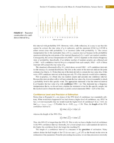
FIGURE 8-1 Repeated
construction of a confi-
dence interval for μ. 1 2 3 4 5 6 7 8 9 10 11 12 13 14 15 16
Interval number

this interval with probability 0.95. However, with a little relection, it is easy to see that this
cannot be correct; the true value of μ is unknown, and the statement 63 84. ≤ μ ≤ 65.08 is
either correct (true with probability 1) or incorrect (false with probability 1). The correct
interpretation lies in the realization that a CI is a random interval because in the probability
statement deining the end-points of the interval (Equation 8-2), L and U are random variables.
Consequently, the correct interpretation of a 100 1 − ≠ )% CI depends on the relative frequency
(
view of probability. Speciically, if an ininite number of random samples are collected and
a 100 1 − ≠ )% conidence interval for μ is computed from each sample, 100 1 − ≠ )% of these
(
(
intervals will contain the true value of μ.
The situation is illustrated in Fig. 8-1, which shows several 100 1 − ≠ )% conidence intervals
(
for the mean μ of a normal distribution. The dots at the center of the intervals indicate the point
estimate of μ (that is, x). Notice that one of the intervals fails to contain the true value of μ. If this
were a 95% conidence interval, in the long run only 5% of the intervals would fail to contain μ.
Now in practice, we obtain only one random sample and calculate one conidence interval.
Because this interval either will or will not contain the true value of μ, it is not reasonable to attach
a probability level to this speciic event. The appropriate statement is that the observed interval
(
[ , ] brackets the true value of μ with conidence 100 1 − ≠ This statement has a frequency
).
l
u
interpretation; that is, we do not know whether the statement is true for this speciic sample, but
the method used to obtain the interval [ , ] yields correct statements 100 1 − ≠ )% of the time.
(
l
u
Confidence Level and Precision of Estimation
Notice that in Example 8-1, our choice of the 95% level of conidence was essentially arbi-
trary. What would have happened if we had chosen a higher level of conidence, say, 99%? In
fact, is it not reasonable that we would want the higher level of conidence? At α = 0 01. , we
ind z α/2 = z . /0 01 2 = z .0 005 = 2 . ,while for α = 0 05. , z 0 025. = 1 96. Thus, the length of the 95%
8
.
5
conidence interval is
. (
2 1 96σ ) = 3 92σ n
.
n
whereas the length of the 99% CI is
. (
.
2 2 58σ ) = 5 16σ n
n
Thus, the 99% CI is longer than the 95% CI. This is why we have a higher level of conidence
in the 99% conidence interval. Generally, for a ixed sample size n and standard deviation σ,
the higher the conidence level, the longer the resulting CI.
The length of a conidence interval is a measure of the precision of estimation. Many
authors deine the half-length of the CI (in our case z α σ n) as the bound on the error in
/2
estimation of the parameter. From the preceeding discussion, we see that precision is inversely