Page 302 - Applied statistics and probability for engineers

280 Chapter 8/Statistical intervals for a single sample

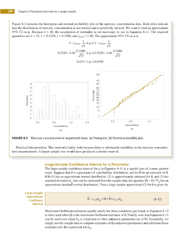
Figure 8-3 presents the histogram and normal probability plot of the mercury concentration data. Both plots indicate
that the distribution of mercury concentration is not normal and is positively skewed. We want to i nd an approximate
95% CI on μ. Because n > 40, the assumption of normality is not necessary to use in Equation 8-11. The required
.
0
quantities are n = 53, x = .5250 ,s = .3486, and z 0 025. = 1 96. The approximate 95% CI on μ is
0
x − z 0 .025 s Ð μ ≤ x + z .0 025 s
n n
.
.
.
.
−
.
+
0 5250 1 96 0 3486 ≤ μ Ð . 0 5250 1 96 0 3486
53 53
.
0 4311≤ μ ≤ 0 6189
.
99
95
9 90
8 80
7 70
60
6 Percentage 50
Frequency 5 30
40
4
20
3 10
2 5
1
1
0
0.0 0.5 1.0 1.5 0.0 0.5 1.0
Concentration Concentration
(b)
(a)
FIGURE 8-3 Mercury concentration in largemouth bass. (a) Histogram. (b) Normal probability plot.

Practical Interpretation: This interval is fairly wide because there is substantial variability in the mercury concentra-
tion measurements. A larger sample size would have produced a shorter interval.

Large-Sample Confi dence Interval for a Parameter

The large-sample conidence interval for μ in Equation 8-11 is a special case of a more general
ˆ
result. Suppose that θ is a parameter of a probability distribution, and let Θ be an estimator of θ.
ˆ
If Θ (1) has an approximate normal distribution, (2) is approximately unbiased for θ, and (3) has
ˆ
standard deviation σ that can be estimated from the sample data, the quantity (Θ − 0) / σ has an
Θ ˆ Θ ˆ
approximate standard normal distribution. Then a large-sample approximate CI for θ is given by
Large-Sample
Approximate ˆ ˆ
θ
Coni dence θ − z α/ σ Θ ˆ ≤ ≤ θ + z α/ σ Θ ˆ (8-12)
2
2
Interval
Maximum likelihood estimators usually satisfy the three conditions just listed, so Equation 8-12
ˆ
is often used when Θ is the maximum likelihood estimator of θ. Finally, note that Equation 8-12
can be used even when σ ˆ is a function of other unknown parameters (or of θ). Essentially, we
Θ
simply use the sample data to compute estimates of the unknown parameters and substitute those
estimates into the expression for σ ˆ .
Θ