Page 299 - Applied statistics and probability for engineers

Section 8-1/Conidence Interval on the Mean of a Normal Distribution, Variance Known 277

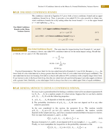
8-1.3 ONE-SIDED CONFIDENCE BOUNDS

The conidence interval in Equation 8-5 gives both a lower conidence bound and an upper

conidence bound for μ. Thus, it provides a two-sided CI. It is also possible to obtain one-

sided conidence bounds for m by setting either the lower bound l = − ∞ or the upper bound
u = ∞ and replacing z α/2 by z α .
One-Sided Coni dence
Bounds on the Mean, A 100 1 − ≠ )% upper-coni dence bound for μ is
(
Variance Known
μ Ð x + z σ α n (8-7)
and a 100 1( − ≠ )% lower-coni dence bound for μ is

l
x − z È n = ≤ μ (8-8)
α

Example 8-3 One-Sided Confi dence Bound The same data for impact testing from Example 8-1 are used

to construct a lower, one-sided 95% conidence interval for the mean impact energy. Recall that
J
x = 64 .46 , σ = 1 , and n = 10. The interval is

σ
x − z α Ð μ
n
− .
.
64 46 1 64 1 ≤ μ
10
63 94 ≤ μ
.
Practical Interpretation: The lower limit for the two-sided interval in Example 8-1 was 63.84. Because z α < z /α 2 , the
lower limit of a one-sided interval is always greater than the lower limit of a two-sided interval of equal coni dence. The
one-sided interval does not bound μ from above so that it still achieves 95% conidence with a slightly larger lower limit.

If our interest is only in the lower limit for μ, then the one-sided interval is preferred because it provides equal coni dence
with a greater limit. Similarly, a one-sided upper limit is always less than a two-sided upper limit of equal coni dence.

8-1.4 GENERAL METHOD TO DERIVE A CONFIDENCE INTERVAL

It is easy to give a general method for inding a conidence interval for an unknown parameter θ.
Let X X 2 ,… , X n be a random sample of n observations. Suppose that we can ind a statistic
1 ,

g X X ,… , X n ; ) with the following properties:
θ
(
, 1
2
θ
1. g X X ,… , X n ; ) depends on both the sample and θ.
(
, 1
2
θ
2. The probability distribution of g X X ,... , X n ; ) does not depend on θ or any other
(
2
, 1
unknown parameter.
In the case considered in this section, the parameter θ = μ. The random variable
σ
g X X ,… , X n ; ) = ( X − μ ) / ( / n) satisi es both conditions; the random variable
μ
(
2
, 1
depends on the sample and on μ, and it has a standard normal distribution because σ is known.
Now we must i nd constants C L and C U so that
P C L ≤ ( 1 2 … n θ) ≤ C U = − α (8-9)
⎤
⎡
1
g X , X , , X ;
⎦
⎣
Because of property 2, C L and C U do not depend on θ. In our example, C L = − α/2 and C U = z α/2 .
z
Finally, we must manipulate the inequalities in the probability statement so that
⎡ ( … ) ≤ θ ≤ ( … )⎤ = 1− α
⎣
P L X , X , , X n1 2 U X , X , , X n1 2 ⎦ (8-10)