Page 300 - Applied statistics and probability for engineers

278 Chapter 8/Statistical intervals for a single sample

This gives L X X ,… , X n ) and U X X ,… , X n ) as the lower and upper coni dence limits
(
(
2
, 1
, 1
2
dei ning the 100 1 − ≠ ) coni dence interval for θ. The quantity g(X , X , …, X ; θ) is often
(
1 2 n
called a pivotal quantity because we pivot on this quantity in Equation 8-9 to produce
σ
Equation 8-10. In our example, we manipulated the pivotal quantity (X − μ ) ( / n ) to
/
,… , X n ) = X − z 2 È n and U ( X X ,… , X n = X + n .
)
obtain L X X( , 1 2 α / , 1 2 z È α/ 2
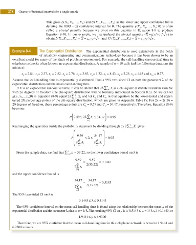
Example 8-4 The Exponential Distribution The exponential distribution is used extensively in the i elds
of reliability engineering and communications technology because it has been shown to be an
excellent model for many of the kinds of problems encountered. For example, the call-handling (processing) time in
telephone networks often follows an exponential distribution. A sample of n = 10 calls had the following durations (in
minutes):
x = 2.84, x = 2.37, x = 7.52, x = 2.76, x = 3.83, x = 1.32, x = 8.43, x = 2.25, x = 1.63 and x = 0.27.
1 2 3 4 5 6 7 8 9 10
Assume that call-handling time is exponentially distributed. Find a 95% two-sided CI on both the parameter λ of the
exponential distribution and the mean call-handling time.
If X is an exponential random variable, it can be shown that 2λ∑ n i= 1 X i is a chi-square distributed random variable
with 2n degrees of freedom (the chi-square distribution will be formally introduced in Section 8.3). So we can let
g x x ,... ; ) in Equation (8-9) equal 2λ∑ n and let C and C in that equation be the lower-tailed and upper-
θ
x n
, 2
( 1
i= 1 X i L U
tailed 2½ percentage points of the chi-square distribution, which are given in Appendix Table IV. For 2n = 2(10) =
20 degrees of freedom, these percentage points are C = 9.59 and C = 34.17, respectively. Therefore, Equation (8-9)
L U
becomes
⎛
⎞
n
P 9 59 2 ∑ X i ≤ 34 17 = 0 95
≤ λ
.
.
⎟
⎜
.
⎠
⎝
=
i 1
Rearranging the quantities inside the probability statement by dividing through by 2∑ n i= 1 X i gives
⎛ ⎞
⎜ 9 59 34 17 ⎟
.
.
P ⎜ n ≤ λ ≤ n ⎟ = 0 95
.
⎜ 2∑ 2∑ ⎟
⎝ i 1= X i i 1= X i ⎠
From the sample data, we i nd that ∑ n x i = 33 22. , so the lower conidence bound on λ is

i=1
.
9 59 = 9 59 =
.
.
n 0 1443
( .
2∑ x i 2 33 22)
i= 1
and the upper conidence bound is

.
34 17 = 34 17 =
.
.
n 0 5143
.
(
2∑ x i 2 33 22)
i= 1
The 95% two-sided CI on λ is
0 1443 ≤ λ ≤ 0 5143
.
.
The 95% coni dence interval on the mean call-handling time is found using the relationship between the mean μ of the
exponential distribution and the parameter λ; that is, μ = 1/ λ. The resulting 95% CI on μ is 1 0 5143 ≤ μ = 1/ ≤ 1 0 1443, or
λ
.
/
/
.
1 9444 ≤ μ ≤ 6 9300
.
.

Therefore, we are 95% conident that the mean call-handling time in this telephone network is between 1.9444 and
6.9300 minutes.