Page 307 - Applied statistics and probability for engineers

Section 8-2/Conidence Interval on the Mean of a Normal Distribution, Variance Known 285

Example 8-6 Alloy Adhesion An article in the journal Materials Engineering (1989, Vol. II, No. 4, pp. 275–
281) describes the results of tensile adhesion tests on 22 U-700 alloy specimens. The load at speci-
men failure is as follows (in megapascals):
19.8 10.1 14.9 7.5 15.4 15.4
15.4 18.5 7.9 12.7 11.9 11.4
11.4 14.1 17.6 16.7 15.8
19.5 8.8 13.6 11.9 11.4
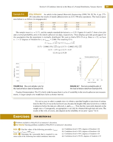
The sample mean is x = 13.71, and the sample standard deviation is s = 3.55. Figures 8-6 and 8-7 show a box plot
and a normal probability plot of the tensile adhesion test data, respectively. These displays provide good support for

the assumption that the population is normally distributed. We want to ind a 95% CI on μ. Since n = 22, we have
n – 1 = 21 degrees of freedom for t, so t = 2.080. The resulting CI is
0.025,21
x − t / ,nα 2 −1 s n Ð μ ≤ x+ t / ,nα 2 −1 s n
. (
.
+
−
13 71 2 080 3 55) 22 ≤ μ Ð 13 71 2 080 3 55) 22
.
.
(
.
.
−
+
13 71 1 57 Ð μ ≤ 13 71 1 57
.
.
.
.
12 14 ≤ μ ≤ 15 28
.
.
Normal probability plot
99
95
90
20.5
80
70
18.0 Percent 60
50
Load at failure 15.5 30
40
20
13.0
10
10.5 5
1
8.0 5 10 15 20 25
Load at failure
FIGURE 8-6 Box and whisker plot for FIGURE 8-7 Normal probability plot of
the load at failure data in Example 8-5. the load at failure data from Example 8-5.
Practical Interpretation: The CI is fairly wide because there is a lot of variability in the tensile adhesion test measure-
ments. A larger sample size would have led to a shorter interval.

It is not as easy to select a sample size n to obtain a speciied length (or precision of estima-
tion) for this CI as it was in the known-σ case, because the length of the interval involves s (which
−1 . Note that the t-percentile depends on the
is unknown before the data are collected), n, and t / ,nα 2
sample size n. Consequently, an appropriate n can only be obtained through trial and error. The
results of this will, of course, also depend on the reliability of our prior “guess” for σ.
Exercises FOR SECTION 8-2
Problem available in WileyPLUS at instructor’s discretion.
Tutoring problem available in WileyPLUS at instructor’s discretion

8-24. Find the values of the following percentiles: t , (a) Conidence level = 95%, degrees of freedom = 12
0.025,15

t , t , t , and t . (b) Conidence level = 95%, degrees of freedom = 24
0.05,10 0.10,20 0.005,25 0.001,30

8-25. Determine the t-percentile that is required to con- (c) Conidence level = 99%, degrees of freedom = 13

struct each of the following two-sided coni dence intervals: (d) Conidence level = 99.9%, degrees of freedom = 15