Page 90 - Applied statistics and probability for engineers

68 Chapter 3/Discrete Random Variables and Probability Distributions

Example 3-4 Digital Channel There is a chance that a bit transmitted through a digital transmission channel
is received in error. Let X equal the number of bits in error in the next four bits transmitted. The
possible values for X are {0, 1, 2, 3, 4}. Based on a model for the errors that is presented in the following section, prob-
abilities for these values will be determined. Suppose that the probabilities are
(
(
.
.
P X = ) =0 0 6561 P X = ) =1 0 2916
(
(
.
P X = ) =2 0 0486 P X = ) =3 0 0036
.
( =
P X = ) 4 = 0 0001.
The probability distribution of X is specii ed by the possible values along with the probability of each. A graphical
description of the probability distribution of X is shown in Fig. 3-1.
Practical Interpretation: A random experiment can often be summarized with a random variable and its distribution.
The details of the sample space can often be omitted.
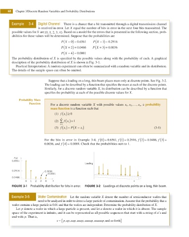
Suppose that a loading on a long, thin beam places mass only at discrete points. See Fig. 3-2.
The loading can be described by a function that speciies the mass at each of the discrete points.

Similarly, for a discrete random variable X, its distribution can be described by a function that

speciies the probability at each of the possible discrete values for X.
Probability Mass
Function For a discrete random variable X with possible values x , x ,… , x n , a probability
1
2
mass function is a function such that
(1) f x i ( ) ≥ 0
n
(2) ∑ f x i ( ) = 1
i=1
P X = )
(3) f x i ( ) = ( x i (3-1)

(
For the bits in error in Example 3-4, f 0 ( ) = 0 6561 , f 1 ( ) = 0 2916 , f 2 ( ) = 0 0486 , f 3) =
.
.
.
0 0036, and f 4 ( ) = 0 0001. Check that the probabilities sum to 1.
.
.
f (x)
0.6561
Loading
0.2916 0.0036
0.0001
0.0486
0 1 2 3 4 x x
FIGURE 3-1 Probability distribution for bits in error. FIGURE 3-2 Loadings at discrete points on a long, thin beam.

Example 3-5 Wafer Contamination Let the random variable X denote the number of semiconductor wafers that
need to be analyzed in order to detect a large particle of contamination. Assume that the probability that a
wafer contains a large particle is 0.01 and that the wafers are independent. Determine the probability distribution of X.
Let p denote a wafer in which a large particle is present, and let a denote a wafer in which it is absent. The sample

space of the experiment is ininite, and it can be represented as all possible sequences that start with a string of a’s and
end with p. That is,
s = { p,ap,aap,aaap,aaaap,aaaaap,and so forth }