Page 93 - Applied statistics and probability for engineers

Section 3-3/Cumulative Distribution Functions 71

3-3 Cumulative Distribution Functions

An alternate method for describing a random variable’s probability distribution is with cumu-
lative probabilities such as P X ≤ x). Furthermore, cumulative probabilities can be used to i nd
(
the probability mass function of a discrete random variable. Consider the following example.

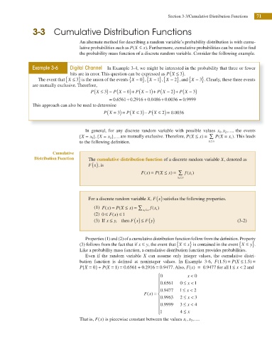
Example 3-6 Digital Channel In Example 3-4, we might be interested in the probability that three or fewer
(
bits are in error. This question can be expressed as P X ≤ ) 3 .
{
The event that X ≤ } 3 is the union of the events X = } { = } 1 , X { = 2 , } and X = } 3 . Clearly, these three events
{
{
, X
0
are mutually exclusive. Therefore,
(
P X = ) + (
P X = ) + (
P X ≤ ) = ( 0 P X = ) + ( 2 P X = ) 3
3
1
= 0 6561 0 2916 0 0486 0.00036 = 0 9999
+
+
+
.
.
.
.
This approach can also be used to determine
(
P X ≤ ) − (
P X = ) = ( 3 P X Ð ) = 0 0036
3
2
.
1 ,
In general, for any discrete random variable with possible values x x 2 ,…, the events
{X = x 1 }, {X = x 2 },… are mutually exclusive. Therefore, P X( ≤ x) = ∑ P X = x i ). This leads
(
to the following dei nition. x i ≤ x
Cumulative
Distribution Function The cumulative distribution function of a discrete random variable X, denoted as
(
F x , ) is
F x) = P X ≤ x) = ∑ f x i )
(
(
(
x i ≤ x
For a discrete random variable X, (
F x) satisies the following properties.
(1) F x( ) = P X ≤ x) = ∑ x i ≤ x f x i )
(
(
(2) 0 ≤ F x( ) ≤ 1
( ) ≤ ( ) y
(3) If x ≤ y, then F x F (3-2)
Properties (1) and (2) of a cumulative distribution function follow from the dei nition. Property
{
{
(3) follows from the fact that if x ≤ y, the event that X ≤ x} is contained in the event X ≤ y}.
Like a probability mass function, a cumulative distribution function provides probabilities.
Even if the random variable X can assume only integer values, the cumulative distri-
bution function is dei ned at noninteger values. In Example 3-6, F(1.5) = P (X ≤ 1.5) =
P X = 0} + P X = 1) = 0.6561 + 0.2916 = 0.9477. Also, F x( ) = 0 9477 for all 1 ≤ x < 2 and
(
{
.
⎧0 x < 0
⎪ ≤
⎪ . 0 6561 0 x < 1
⎪ . 0 9477 1 ≤ x < 2
F x) = ⎨ ⎨
(
⎪ . 0 9963 2 ≤ x < 3
⎪ . 0 9999 3 ≤ x < 4
⎪
⎩ 1 4 ≤ x
1 ,
That is, F x( ) is piecewise constant between the values x x 2 ,….