Page 97 - Applied statistics and probability for engineers

Section 3-4/Mean and Variance of a Discrete Random Variable 75

Example 3-9 Digital Channel In Example 3-4, there is a chance that a bit transmitted through a digital trans-
mission channel is received in error. Let X equal the number of bits in error in the next four bits
{
,
,
,
,
transmitted. The possible values for X are 0 1 2 3 4}. Based on a model for the errors presented in the following sec-
tion, probabilities for these values will be determined. Suppose that the probabilities are
(
(
(
0
P X = ) = 0 6561. P X = ) = 0 0486. P X = ) = 0 0001.
4
2
( P(
.
.
3
P X = ) =1 0 2916 P X = ) = 0 0036
Now
E X
μ = ( ) = f0 ( ) + ( ) + ( ) + ( ) + f0 f 1 1 f 2 2 f 3 3 4 ( ) 4
4 0 0001)
. (
= ( 0 0 6561 ) + ( 1 0 2916. ) + 2 0 0486. ( 0 ) + 3 0 0036) + ( .
.
= 0 4
.
Although X never assumes the value 0.4, the weighted average of the possible values is 0.4.
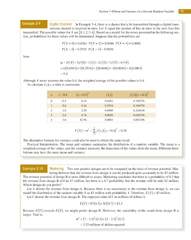
To calculate V X ,( ) a table is convenient.
(
.
.
x x − 0 4 ( x − 0 4 ) 2 f x ( ) f x x )( − 0 4 ) 2
.
0 –0.4 0.16 0.6561 0.104976
1 0.6 0.36 0.2916 0.104976
2 1.6 2.56 0.0486 0.124416
3 2.6 6.76 0.0036 0.024336
4 3.6 12.96 0.0001 0.001296
5 2
V X ( ) = σ = ∑ f x i ( )( x i − 0 4 ) = 0 36.
2
.
i=1
The alternative formula for variance could also be used to obtain the same result.
Practical Interpretation: The mean and variance summarize the distribution of a random variable. The mean is a
weighted average of the values, and the variance measures the dispersion of the values from the mean. Different distri-
butions may have the same mean and variance.

Example 3-10 Marketing Two new product designs are to be compared on the basis of revenue potential. Mar-
keting believes that the revenue from design A can be predicted quite accurately to be $3 million.
The revenue potential of design B is more dificult to assess. Marketing concludes that there is a probability of 0.3 that

the revenue from design B will be $7 million, but there is a 0.7 probability that the revenue will be only $2 million.
Which design do you prefer?
Let X denote the revenue from design A. Because there is no uncertainty in the revenue from design A, we can
model the distribution of the random variable X as $3 million with probability 1. Therefore, E X ( ) = $3 million.
Let Y denote the revenue from design B. The expected value of Y in millions of dollars is

.
E Y ( ) = $7 ( ) + ( ) =$0 3. 2 0 7 $3 .5
Because E Y ( ) exceeds E X ( ), we might prefer design B. However, the variability of the result from design B is
larger. That is,
2
σ = (7 3 5. 2 0 3 − ) ( ) 7. 2 0.
− ) ( ) +(2 3 5.
.
= 5 25 millions of dollars squuared