Page 103 - Applied Statistics Using SPSS, STATISTICA, MATLAB and R

82 3 Estimating Data Parameters

loss of elasticity since the last calibration made at the factory, and exhibiting,
therefore, a permanent deviation (bias) from the correct value; a random parallax
error, corresponding to the evaluation of the gauge needle position, which can be
considered normally distributed around the correct position (variance). The
situation is depicted in Figure 3.1.
The weight measurement can be considered as a “bias + variance” situation. The
bias, or systematic error, is a constant. The source of variance is a random error.

σ

ω w w
bias
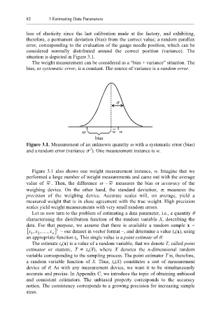
Figure 3.1. Measurement of an unknown quantity ω with a systematic error (bias)
2
and a random error (variance σ ). One measurement instance is w.

Figure 3.1 also shows one weight measurement instance, w. Imagine that we
performed a large number of weight measurements and came out with the average
value of w . Then, the difference ω − w measures the bias or accuracy of the
weighing device. On the other hand, the standard deviation, σ, measures the
precision of the weighing device. Accurate scales will, on average, yield a
measured weight that is in close agreement with the true weight. High precision
scales yield weight measurements with very small random errors.
Let us now turn to the problem of estimating a data parameter, i.e., a quantity θ
characterising the distribution function of the random variable X, describing the
data. For that purpose, we assume that there is available a random sample x =
[ 1 x ,K x , n ]x , ’ − our dataset in vector format −, and determine a value t n(x), using
2
an appropriate function t n. This single value is a point estimate of θ.
The estimate t n(x) is a value of a random variable, that we denote T, called point
estimator or statistic, T ≡ t n(X), where X denotes the n-dimensional random
variable corresponding to the sampling process. The point estimator T is, therefore,
a random variable function of X. Thus, t n(X) constitutes a sort of measurement
device of θ. As with any measurement device, we want it to be simultaneously
accurate and precise. In Appendix C, we introduce the topic of obtaining unbiased
and consistent estimators. The unbiased property corresponds to the accuracy
notion. The consistency corresponds to a growing precision for increasing sample
sizes.