Page 105 - Applied Statistics Using SPSS, STATISTICA, MATLAB and R

84 3 Estimating Data Parameters

w − . 1 96 σ < ω < w + . 1 96 σ , 3.4

allowing us to define the 95% confidence interval for the unknown weight
(parameter) ω given a particular measurement w. (Comparing with expression 3.1
we see that in this case θ is the parameter ω, t 1,1 = w – 1.96σ and t 1,2 = w + 1.96σ.)
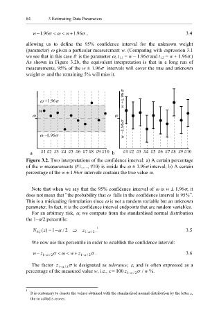
As shown in Figure 3.2b, the equivalent interpretation is that in a long run of
measurements, 95% of the w ± 1.96σ intervals will cover the true and unknown
weight ω and the remaining 5% will miss it.

w +1.96σ
ω +1.96σ

w
ω ω
w −1.96σ

ω −1.96σ

a #1 #2 #3 #4 #5 #6 #7 #8 #9 #10 b #1 #2 #3 #4 #5 #6 #7 #8 #9 #10
Figure 3.2. Two interpretations of the confidence interval: a) A certain percentage
of the w measurements (#1,…, #10) is inside the ω ± 1.96σ interval; b) A certain
percentage of the w ± 1.96σ intervals contains the true value ω.

Note that when we say that the 95% confidence interval of ω is w ± 1.96σ , it
“
does not mean that the probability that ω falls in the confidence interval is 95% . ”
This is a misleading formulation since ω is not a random variable but an unknown
parameter. In fact, it is the confidence interval endpoints that are random variables.
For an arbitrary risk, α, we compute from the standardised normal distribution
the 1–α/2 percentile:

−
N 1 , 0 (z ) = 1 α 2 / ⇒ z 1 α 2 / . 1 3.5
−

We now use this percentile in order to establish the confidence interval:

w − z 1− α 2 σ < ω < w + z 1− α 2 σ . 3.6
/
/

The factor z 1− α 2 σ is designated as tolerance, ε, and is often expressed as a
/
percentage of the measured value w, i.e., ε = 100 z 1− α 2 σ / w %.
/

1
It is customary to denote the values obtained with the standardised normal distribution by the letter z,
the so called z-scores.