Page 283 - Applied Statistics Using SPSS, STATISTICA, MATLAB and R

264 6 Statistical Classification

i(t 1) = i(t 2) = 1×1= 1;
2 1 2
i(t 11) = i(t 12) = = ;
3 3 9
i(t 21) = i(t 22) = 1×0 = 0.

In the automatic generation of binary trees the tree starts at the root node, which
corresponds to the whole training set. Then, it progresses by searching for each
variable the threshold level achieving the maximum decrease of the impurity at
each node. The generation of splits stops when no significant decrease of the
impurity is achieved. It is common practice to use the individual feature values of
the training set cases as candidate threshold values. Sometimes, after generating a
tree automatically, some sort of tree pruning should be performed in order to
remove branches of no interest.
SPSS and STATISTICA have specific commands for designing tree classifiers,
based on univariate splits. The method of exhaustive search for the best univariate
splits is usually called the CRT (also CART or C&RT) method, pioneered by
Breiman, Friedman, Olshen and Stone (see Breiman et al., 1993).

Example 6.17
Q: Use the CR T approach with univariate splits and the Gini index as splitting
criterion in order to derive a decision tree for the Breast Tissue dataset.
Assume equal priors of the classes.
A: Applying the commands for CRT univariate split with the Gini index, described
in Commands 6.3, the tree presented in Figure 6.28 was found with SPSS (same
solution with STATISTICA). The tree shows the split thresholds at each node as
well as the improvement achieved in the Gini index. For instance, the first split
variable PERIM was selected with a threshold level of 1563.84.

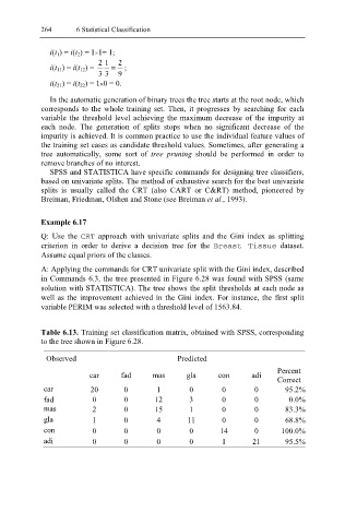
Table 6.13. Training set classification matrix, obtained with SPSS, corresponding
to the tree shown in Figure 6.28.
Observed Predicted
Percent
car fad mas gla con adi
Correct
car 20 0 1 0 0 0 95.2%
fad 0 0 12 3 0 0 0.0%
mas 2 0 15 1 0 0 83.3%
gla 1 0 4 11 0 0 68.8%
con 0 0 0 0 14 0 100.0%
adi 0 0 0 0 1 21 95.5%