Page 36 - Applied Statistics Using SPSS, STATISTICA, MATLAB and R

1.5 Beyond a Reasonable Doubt... 15

to absolute certainty if this number tends to infinite), and that if the jury wanted to
increase the precision (details) of the verdict, it would then lose in degree of
certainty.

Table 1.6. Confidence levels (δ) for the interval estimation of a proportion, when
p ˆ = 0.74, for two different values of the tolerance (ε).
n δ for ε = 0.02 δ for ε = 0.01
50 0.25 0.13
100 0.35 0.18
1000 0.85 0.53
10000 ≈ 1.00 0.98

1.2
δ
1.0

0.8 ε=0.04
ε=0.02
0.6
ε=0.01
0.4
0.2
n
0.0
0 500 1000 1500 2000 2500 3000 3500 4000

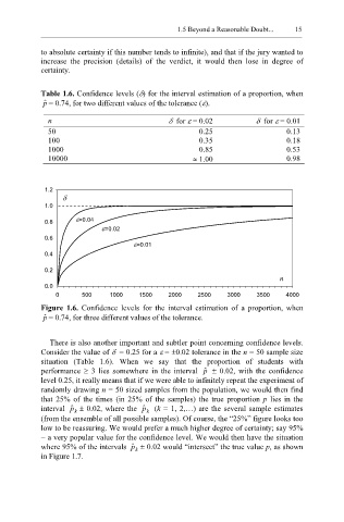
Figure 1.6. Confidence levels for the interval estimation of a proportion, when
p ˆ = 0.74, for three different values of the tolerance.

There is also another important and subtler point concerning confidence levels.
Consider the value of δ = 0.25 for a ε = ±0.02 tolerance in the n = 50 sample size
situation (Table 1.6). When we say that the proportion of students with
performance ≥ 3 lies somewhere in the interval p ˆ ± 0.02, with the confidence
level 0.25, it really means that if we were able to infinitely repeat the experiment of
randomly drawing n = 50 sized samples from the population, we would then find
that 25% of the times (in 25% of the samples) the true proportion p lies in the
interval p ˆ ± 0.02, where the p ˆ (k = 1, 2,…) are the several sample estimates
k
k
(from the ensemble of all possible samples). Of course, the “25%” figure looks too
low to be reassuring. We would prefer a much higher degree of certainty; say 95%
− a very popular value for the confidence level. We would then have the situation
where 95% of the intervals p ˆ ± 0.02 would “intersect” the true value p, as shown
k
in Figure 1.7.