Page 33 - Applied Statistics Using SPSS, STATISTICA, MATLAB and R

12 1 Introduction

1 P(x)
F(x)
0.8
0.6
0.4
0.2
x
0
1 2 3 4 5
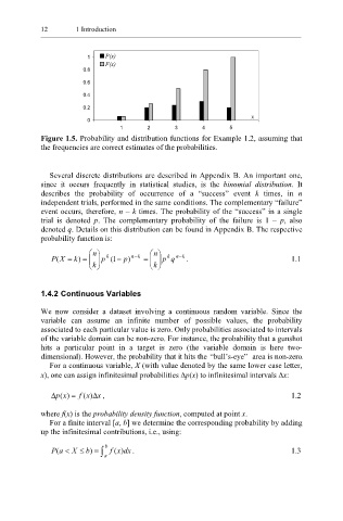
Figure 1.5. Probability and distribution functions for Example 1.2, assuming that
the frequencies are correct estimates of the probabilities.

Several discrete distributions are described in Appendix B. An important one,
since it occurs frequently in statistical studies, is the binomial distribution. It
describes the probability of occurrence of a “success” event k times, in n
independent trials, performed in the same conditions. The complementary “failure”
event occurs, therefore, n – k times. The probability of the “success” in a single
trial is denoted p. The complementary probability of the failure is 1 – p, also
denoted q. Details on this distribution can be found in Appendix B. The respective
probability function is:

 n  n
k
P( X = k =)     p 1( − p) n− k =     p k q n− k . 1.1
 k   k 

1.4.2 Continuous Variables

We now consider a dataset involving a continuous random variable. Since the
variable can assume an infinite number of possible values, the probability
associated to each particular value is zero. Only probabilities associated to intervals
of the variable domain can be non-zero. For instance, the probability that a gunshot
hits a particular point in a target is zero (the variable domain is here two-

dimensional). However, the probability that it hits the “bull’s-eye” area is non-zero .

For a continuous variable, X (with value denoted by the same lower case letter,
x), one can assign infinitesimal probabilities ∆p(x) to infinitesimal intervals ∆x:

∆ p( x = f ( x ∆ x , 1.2
)
)

where f(x) is the probability density function, computed at point x.
For a finite interval [a, b] we determine the corresponding probability by adding
up the infinitesimal contributions, i.e., using:

P( a < X ≤ b) = ∫ a b f ( x) dx . 1.3