Page 30 - Applied Statistics Using SPSS, STATISTICA, MATLAB and R

1.3 Random Variables 9

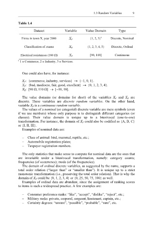
Table 1.4
Dataset Variable Value Domain Type

Firms in town X, year 2000 X F {1, 2, 3} a Discrete, Nominal

Classification of exams X E {1, 2, 3, 4, 5} Discrete, Ordinal

Electrical resistances (100 Ω) X R [90, 110] Continuous
a 1 ≡ Commerce, 2 ≡ Industry, 3 ≡ Services.

One could also have, for instance:

X F: {commerce, industry, services} → {−1, 0, 1}.
X E: {bad, mediocre, fair, good, excellent} → {0, 1, 2, 3, 4}.
X R: [90 Ω, 110 Ω] → [−10, 10].

The value domains (or domains for short) of the variables X F and X E are
discrete. These variables are discrete random variables. On the other hand,
variable X R is a continuous random variable.
The values of a nominal (or categorial) discrete variable are mere symbols (even
if we use numbers) whose only purpose is to distinguish different categories (or
classes). Their value domain is unique up to a biunivocal (one-to-one)
transformation. For instance, the domain of X F could also be codified as {A, B, C}
or {I, II, III}.
Examples of nominal data are:

– Class of animal: bird, mammal, reptile, etc.;
– Automobile registration plates;
– Taxpayer registration numbers.

The only statistics that make sense to compute for nominal data are the ones that
are invariable under a biunivocal transformation, namely: category counts;
frequencies (of occurrence); mode (of the frequencies).
The domain of ordinal discrete variables, as suggested by the name, supports a
total order relation (“larger than” or “smaller than”). It is unique up to a strict
monotonic transformation (i.e., preserving the total order relation). That is why the
domain of X E could be {0, 1, 2, 3, 4} or {0, 25, 50, 75, 100} as well.
Examples of ordinal data are abundant, since the assignment of ranking scores
to items is such a widespread practice. A few examples are:

– Consumer preference ranks: “like”, “accept”, “dislike”, “reject”, etc.;
– Military ranks: private, corporal, sergeant, lieutenant, captain, etc.;
– Certainty degrees: “unsure”, “possible”, “probable”, “sure”, etc.