Page 25 - Applied Statistics Using SPSS, STATISTICA, MATLAB and R

4 1 Introduction

precision of the result cannot be properly controlled by the precision of the causes.
To illustrate this, let us consider the following formula used as a model of
population growth in ecology studies, where p(n) ∈ [0, 1] is the fraction of a
limiting number of population of a species at instant n, and k is a constant that
depends on ecological conditions, such as the amount of food present:

p n+ 1 = p n 1 ( + 1 ( k − p n )) , k > 0.

Imagine we start (n = 1) with a population percentage of 50% (p 1 = 0.5) and
wish to know the percentage of population at the following three time instants,
with k = 1.9:

p 2 = p 1(1+1.9 x (1− p 1)) = 0.9750
p 3 = p 2(1+1.9 x (1− p 2)) = 1.0213
p 4 = p 3(1+1.9 x (1− p 3)) = 0.9800

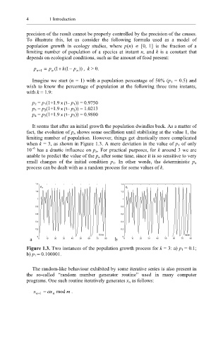
It seems that after an initial growth the population dwindles back. As a matter of
fact, the evolution of p n shows some oscillation until stabilising at the value 1, the
limiting number of population. However, things get drastically more complicated
when k = 3, as shown in Figure 1.3. A mere deviation in the value of p 1 of only
−6
10 has a drastic influence on p n. For practical purposes, for k around 3 we are
unable to predict the value of the p n after some time, since it is so sensitive to very
small changes of the initial condition p 1. In other words, the deterministic p n
process can be dealt with as a random process for some values of k.

1.4 1.4
p n p
n
1.2 1.2
1 1
0.8 0.8
0.6 0.6
0.4 0.4
0.2 0.2
time time
a 0 0 10 20 30 40 50 60 70 80 b 0 0 10 20 30 40 50 60 70 80
Figure 1.3. Two instances of the population growth process for k = 3: a) p 1 = 0.1;
b) p 1 = 0.100001.

The random-like behaviour exhibited by some iterative series is also present in
the so-called “random number generator routine” used in many computer
programs. One such routine iteratively generates x n as follows:

x n 1 = α x mod m .
+
n