Page 32 - Applied Statistics Using SPSS, STATISTICA, MATLAB and R

1.4 Probabilities and Distributions 11

Probability, since for the first time, mathematical grounds were established and the
application of probability to statistics was presented. The notion of probability is
originally associated with the notion of frequency of occurrence of one out of k
events in a sequence of trials, in which each of the events can occur by pure
chance.
Let us assume a sample dataset, of size n, described by a discrete variable, X.
Assume further that there are k distinct values x i of X each one occurring n i times.
We define:

– Absolute frequency of x i: n i ;
n k
n .
– Relative frequency (or simply frequency of x i): f = i with n = ∑ i
i
n = i 1
In the classic frequency interpretation, probability is considered a limit, for large
n, of the relative frequency of an event: P i ≡ P (X = x i ) = lim n → ∞ f i [ ∈ ] 1 , 0 . In
Appendix A, a more rigorous definition of probability is presented, as well as
properties of the convergence of such a limit to the probability of the event (Law of
Large Numbers), and the justification for computing (XP = x i ) as the ratio of the
“
”
number of favourable events over the number of possible events when the event
composition of the random experiment is known beforehand. For instance, the
probability of obtaining two heads when tossing two coins is ¼ since only one out
of the four possible events (head-head, head-tail, tail-head, tail-tail) is favourable.
As exemplified in Appendix A, one often computes probabilities of events in this
way, using enumerative and combinatorial techniques.
The values of P i constitute the probability function values of the random
variable X, denoted P(X). In the case the discrete random variable is an ordinal
variable the accumulated sum of P i is called the distribution function, denoted
F(X). Bar graphs are often used to display the values of probability and distribution
functions of discrete variables.
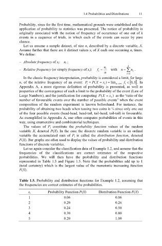
Let us again consider the classification data of Example 1.2, and assume that the
frequencies of the classifications are correct estimates of the respective
probabilities. We will then have the probability and distribution functions
represented in Table 1.5 and Figure 1.5. Note that the probabilities add up to 1
(total certainty) which is the largest value of the monotonic increasing function
F(X).

Table 1.5. Probability and distribution functions for Example 1.2, assuming that
the frequencies are correct estimates of the probabilities.
x i Probability Function P(X) Distribution Function F(X)
1 0.06 0.06
2 0.20 0.26
3 0.24 0.50
4 0.30 0.80
5 0.20 1.00