Page 37 - Applied Statistics Using SPSS, STATISTICA, MATLAB and R

16 1 Introduction

Imagine then that we were dealing with random samples from a random
experiment in which we knew beforehand that a “success” event had a p = 0.75
probability of occurring. It could be, for instance, randomly drawing balls with
replacement from an urn containing 3 black balls and 1 white “failure” ball. Using
the normal approximation of P n, one can compute the needed sample size in order
to obtain the 95% confidence level, for an ε = ±0.02 tolerance. It turns out to be
n ≈ 1800. We now have a sample of 1800 drawings of a ball from the urn, with an
estimated proportion, say ˆ p , of the success event. Does this mean that when
0
dealing with a large number of samples of size n = 1800 with estimates p ˆ (k = 1,
k
2,…), 95% of the p ˆ will lie somewhere in the interval ˆ p ± 0.02? No. It means,
k
0
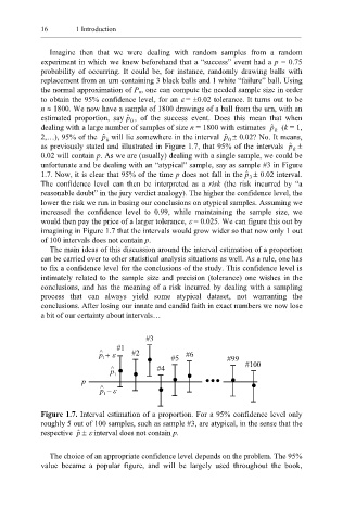
as previously stated and illustrated in Figure 1.7, that 95% of the intervals p ˆ ±
k
0.02 will contain p. As we are (usually) dealing with a single sample, we could be
unfortunate and be dealing with an “atypical” sample, say as sample #3 in Figure
1.7. Now, it is clear that 95% of the time p does not fall in the ˆ p ± 0.02 interval.
3
The confidence level can then be interpreted as a risk (the risk incurred by “a
reasonable doubt” in the jury verdict analogy). The higher the confidence level, the
lower the risk we run in basing our conclusions on atypical samples. Assuming we
increased the confidence level to 0.99, while maintaining the sample size, we
would then pay the price of a larger tolerance, ε = 0.025. We can figure this out by
imagining in Figure 1.7 that the intervals would grow wider so that now only 1 out
of 100 intervals does not contain p.
The main ideas of this discussion around the interval estimation of a proportion
can be carried over to other statistical analysis situations as well. As a rule, one has
to fix a confidence level for the conclusions of the study. This confidence level is
intimately related to the sample size and precision (tolerance) one wishes in the
conclusions, and has the meaning of a risk incurred by dealing with a sampling
process that can always yield some atypical dataset, not warranting the
conclusions. After losing our innate and candid faith in exact numbers we now lose
a bit of our certainty about intervals…

#3
#1
^ 1 + ε #2 #5 #6 #99
p
p ^ 1 #4 ... #100
p
^ 1 − ε
p

Figure 1.7. Interval estimation of a proportion. For a 95% confidence level only
roughly 5 out of 100 samples, such as sample #3, are atypical, in the sense that the
respective p ˆ ± ε interval does not contain p.

The choice of an appropriate confidence level depends on the problem. The 95%
value became a popular figure, and will be largely used throughout the book,