Page 95 - Applied Statistics Using SPSS, STATISTICA, MATLAB and R

74 2 Presenting and Summarising the Data

Note that the denominator of φ will ensure a value in the interval [−1, 1] as with
the correlation coefficient, with +1 representing a perfect positive association and
–1 a perfect negative association. As a matter of fact the phi coefficient is a special
case of the Pearson correlation.

Table 2.11. A general cross table for the bivariate dichotomous case.
y 1 y 2 Total
x 1 a b a + b
x 2 c d c + d
Total a + c b + d a + b + c + d

Example 2.9
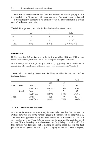
Q: Consider the 2×2 contingency table for the variables SEX and INIT of the
Freshmen dataset, shown in Table 2.12. Compute their phi coefficient.
A: The computed value of phi using 2.26 is 0.15, suggesting a very low degree of
association. The significance of the phi values will be discussed in Chapter 5.

Table 2.12. Cross table (obtained with SPSS) of variables SEX and INIT of the
freshmen dataset.
INIT Total
yes no
SEX male Count 91 5 96
% of Total 69.5% 3.8% 73.3%
female Count 30 5 35
% of Total 22.9% 3.8% 26.7%
Total Count 121 10 131
% of Total 92.4% 7.6% 100.0%

2.3.6.2 The Lambda Statistic

Another useful measure of association, for multivariate nominal data, attempts to
evaluate how well one of the variables predicts the outcome of the other variable.
This measure is applicable to any nominal variables, either dichotomous or not. We
will explain it using Table 2.4, by attempting to estimate the contribution of
variable SEX in lowering the prediction error of Q4 (“liking to be initiated”). For
that purpose, we first note that if nothing is known about the sex, the best
prediction of the Q4 outcome is the “agree” category, the so-called modal category,