Page 93 - Applied Statistics Using SPSS, STATISTICA, MATLAB and R

72 2 Presenting and Summarising the Data

+
where the N is the sum of all counts below and to the right of the ijth cell, and
ij
−
the N is the sum of all counts below and to the left of the ijth cell.
ij
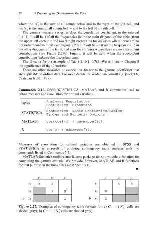
The gamma measure varies, as does the correlation coefficient, in the interval
[−1, 1]. It will be 1 if all the frequencies lie in the main diagonal of the table (from
the upper left corner to the lower right corner), as for all cases where there are no
discordant contributions (see Figure 2.27a). It will be –1 if all the frequencies lie in
the other diagonal of the table, and also for all cases where there are no concordant
contributions (see Figure 2.27b). Finally, it will be zero when the concordant
contributions balance the discordant ones.
The G value for the example of Table 2.10 is 0.785. We will see in Chapter 5
the significance of the G statistic.
There are other measures of association similar to the gamma coefficient that
are applicable to ordinal data. For more details the reader can consult e.g. (Siegel S,
Castellan Jr NJ, 1988).

Commands 2.10. SPSS, STATISTICA, MATLAB and R commands used to
obtain measures of association for ordinal variables.

SPSS Analyze; Descriptive
Statistics; Crosstabs
STATISTICA Statistics; Basic Statistics/Tables;
Tables and Banners; Options

MATLAB corrcoef(x) ; gammacoef(t)
R cor(x) ; gammacoef(t)

Measures of association for ordinal variables are obtained in SPSS and
STATISTICA as a result of applying contingency table analysis with the
commands listed in Commands 5.7.
MATLAB Statistics toolbox and R stats package do not provide a function for
computing the gamma statistic. We provide, however, MATLAB and R functions
for that purpose in the book CD (see Appendix F).

y 1 y 2 y 3 y 1 y 2 y 3
x 1 x x x 1 x x

x 2 x x x 2 x
a x 3 x b x 3 x

−
Figure 2.27. Examples of contingency table formats for: a) G = 1 ( N cells are
ij
+
shaded gray); b) G = –1 ( N cells are shaded gray).
ij