Page 88 - Applied Statistics Using SPSS, STATISTICA, MATLAB and R

2.3 Summarising the Data 67

where s XY, the sample covariance of X and Y, is computed as:

n
s XY = ∑ n 1 = i (x i − x ( ) y i − ) y /( − ) 1 . 2.19

Note that the correlation coefficient (also known as Pearson correlation) is a
dimensionless measure of the degree of linear association of two r.v., with value in
the interval [−1, 1], with:

0 : No linear association (X and Y are linearly uncorrelated);
1 : Total linear association, with X and Y varying in the same direction;
−1: Total linear association, with X and Y varying in the opposite direction.

Figure 2.26 shows scatter plots exemplifying several situations of correlation.
Figure 2.26f illustrates a situation where, although there is an evident association
between X and Y, the correlation coefficient fails to measure it since X and Y are
not linearly associated.
Note that, as described in Appendix A (section A.8.2), adding a constant or
multiplying by a constant any or both variables does not change the magnitude of
the correlation coefficient. Only a change of sign can occur if one of the
multiplying constants is negative.
The correlation coefficients can be arranged, in general, into a symmetrical
correlation matrix, where each element is the correlation coefficient of the
respective column and row variables.

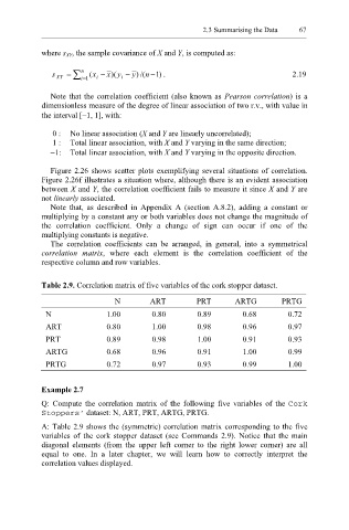
Table 2.9. Correlation matrix of five variables of the cork stopper dataset.

N ART PRT ARTG PRTG
N 1.00 0.80 0.89 0.68 0.72
ART 0.80 1.00 0.98 0.96 0.97
PRT 0.89 0.98 1.00 0.91 0.93
ARTG 0.68 0.96 0.91 1.00 0.99
PRTG 0.72 0.97 0.93 0.99 1.00

Example 2.7

Q: Compute the correlation matrix of the following five variables of the Cork
Stoppers’ dataset: N, ART, PRT, ARTG, PRTG.
A: Table 2.9 shows the (symmetric) correlation matrix corresponding to the five
variables of the cork stopper dataset (see Commands 2.9). Notice that the main
diagonal elements (from the upper left corner to the right lower corner) are all
equal to one. In a later chapter, we will learn how to correctly interpret the
correlation values displayed.