Page 87 - Applied Statistics Using SPSS, STATISTICA, MATLAB and R

66 2 Presenting and Summarising the Data

There are no functions in the R stats package to compute the skewness and
kurtosis. We provide, however, as stated in Commands 2.8, R functions for that
purpose in text file format in the book CD (see Appendix F). The only thing to be
done is to copy the function text from the file and paste it in the R console, as in
the following example:

> skewness <- function(x){
+ n <- length(x)
+ y < - ( x - m e a n ( x ) ) ^ 3
+ n*sum(y)/((n-1)*(n-2)*sd(x)^3)
+ }
> skewness(PRT)
[1] 0.592342

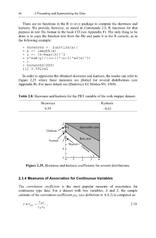
In order to appreciate the obtained skewness and kurtosis, the reader can refer to
Figure 2.25 where these measures are plotted for several distributions (see
Appendix B). For more details see (Dudewicz EJ, Mishra SN, 1988).

Table 2.8. Skewness and kurtosis for the PRT variable of the cork stopper dataset.
Skewness Kurtosis
0.59 −0.63

-2
k Impossible area
Uniform 0

Beta area
Normal 2
Student t
4 Gamma
g
6
0 1 2 3 4
Figure 2.25. Skewness and kurtosis coefficients for several distributions.

2.3.4 Measures of Association for Continuous Variables
The correlation coefficient is the most popular measure of association for
continuous type data. For a dataset with two variables, X and Y, the sample
estimate of the correlation coefficient ρ XY (see definition in A.8.2) is computed as:
s
r ≡ r XY = XY , 2.18
s X s Y