Page 168 - Artificial Intelligence for Computational Modeling of the Heart

140 Chapter 4 Data-driven reduction of cardiac models

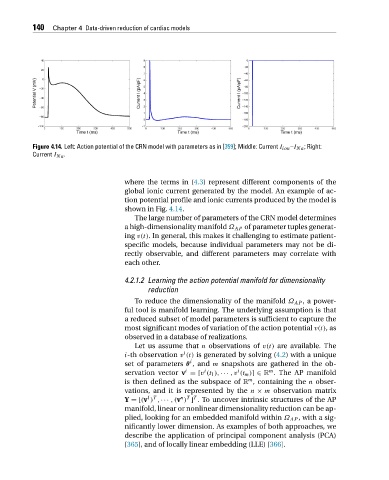
Figure 4.14. Left: Action potential of the CRN model with parameters as in [359]; Middle: Current I ion –I Na ; Right:
Current I Na .

where the terms in (4.3) represent different components of the
global ionic current generated by the model. An example of ac-
tion potential profile and ionic currents produced by the model is
showninFig. 4.14.
The large number of parameters of the CRN model determines
a high-dimensionality manifold Ω AP of parameter tuples generat-
ing v(t). In general, this makes it challenging to estimate patient-
specific models, because individual parameters may not be di-
rectly observable, and different parameters may correlate with
each other.

4.2.1.2 Learning the action potential manifold for dimensionality
reduction
To reduce the dimensionality of the manifold Ω AP ,apower-
ful tool is manifold learning. The underlying assumption is that
a reduced subset of model parameters is sufficient to capture the
most significant modes of variation of the action potential v(t),as
observed in a database of realizations.
Let us assume that n observations of v(t) are available. The
i
i-th observation v (t) is generated by solving (4.2) with a unique
i
set of parameters θ ,and m snapshots are gathered in the ob-
m
i
i
i
servation vector v =[v (t 1 ),··· ,v (t m )]∈ R . The AP manifold
m
is then defined as the subspace of R , containing the n obser-
vations, and it is represented by the n × m observation matrix
1 T
n T T
Y =[(v ) ,··· ,(v ) ] . To uncover intrinsic structures of the AP
manifold, linear or nonlinear dimensionality reduction can be ap-
plied, looking for an embedded manifold within Ω AP , with a sig-
nificantly lower dimension. As examples of both approaches, we
describe the application of principal component analysis (PCA)
[365], and of locally linear embedding (LLE) [366].