Page 172 - Artificial Intelligence for Computational Modeling of the Heart

144 Chapter 4 Data-driven reduction of cardiac models

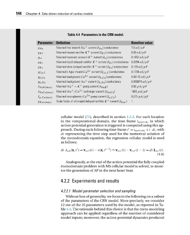
Table 4.4 Parameters in the CRN model.

Parameter Definition Baseline value
+
g Na Maximal fast inward Na current (I Na ) conductance 7.8 nS/pF
g K1 Maximal inward rectifier K + current (I K1 ) conductance 0.09 nS/pF
g to Maximal transient outward K + current (I to ) conductance 0.1652 nS/pF
g Kr Maximal rapid delayed rectifier K + current (I Kr ) conductance 0.0294 nS/pF
g Ks Maximal slow delayed rectifier K + current (I Ks ) conductance 0.129 nS/pF
g Ca,L Maximal L-type inward Ca 2+ current (I Ca,L ) conductance 0.1238 nS/pF
g b,Ca Maximal background Ca 2+ current (I b,Ca ) conductance 0.00113 nS/pF
+
g b,Na Maximal background Na current (I b,Na ) conductance 0.000674 nS/pF
+
I NaK(max) Maximal Na − K + pump current (I NaK ) 0.60 pA/pF
+
I NaCa(max) Maximal Na /Ca 2+ exchanger current (I NaCa ) 1600 pA/pF
I p,Ca(max) Maximal sarcoplasmic Ca 2+ pump current (I p,Ca ) 0.275 pA/pF
g Kur(max) Scale factor of ultrarapid delayed rectifier K + current (I Kur ) 1

cellular model [71], described in section 1.2.2. For each location
in the computational domain, the time frame t upstroke in which
action potential generation is triggered is computed using this ap-
i
proach. During each following time frame t = t upstroke +i ·dt, with
dt representing the time step used for the numerical solution of
the monodomain equation, the regression cellular model is used
as follows:
i
dt J ion (x,t ) = v ref (i) − v(x,t i−1 ) ≈ v ref (i) − v ref (i − 1) = dt J ref (i).
(4.6)

Analogously, at the end of the action potential the fully coupled
monodomain problem with MS cellular model is solved, to moni-
tor the generation of AP in the next heart beat.

4.2.2 Experiments and results

4.2.2.1 Model parameter selection and sampling
Without loss of generality, we focus in the following on a subset
of the parameters of the CRN model. More precisely, we consider
12 out of the 35 parameters used by the model, as reported in Ta-
ble 4.4. The rationale behind this choice is that the meta-modeling
approach can be applied regardless of the number of considered
model inputs; moreover, the action potential dynamics produced