Page 192 - Artificial Intelligence for Computational Modeling of the Heart

164 Chapter 5 Machine learning methods for robust parameter estimation

2
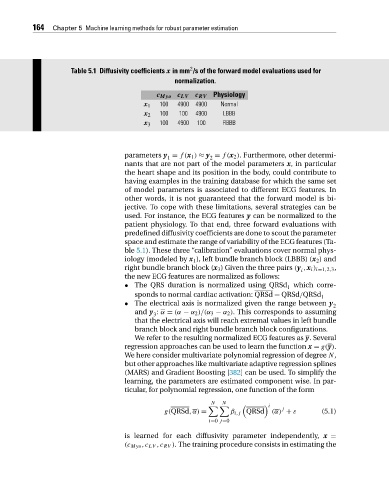
Table 5.1 Diffusivity coefficients x in mm /s of the forward model evaluations used for
normalization.

c Myo c LV c RV Physiology
x 1 100 4900 4900 Normal
x 2 100 100 4900 LBBB
x 3 100 4900 100 RBBB

parameters y = f(x 1 ) ≈ y = f(x 2 ). Furthermore, other determi-
1 2
nants that are not part of the model parameters x, in particular
the heart shape and its position in the body, could contribute to
having examples in the training database for which the same set
of model parameters is associated to different ECG features. In
other words, it is not guaranteed that the forward model is bi-
jective. To cope with these limitations, several strategies can be
used. For instance, the ECG features y can be normalized to the
patient physiology. To that end, three forward evaluations with
predefined diffusivity coefficients are done to scout the parameter
space and estimate the range of variability of the ECG features (Ta-
ble 5.1). These three “calibration” evaluations cover normal phys-
iology (modeled by x 1 ), left bundle branch block (LBBB) (x 2 )and
right bundle branch block (x 3 ) Given the three pairs (y ,x i ) i=1,2,3 ,
i
the new ECG features are normalized as follows:
• The QRS duration is normalized using QRSd which corre-
1
sponds to normal cardiac activation: QRSd = QRSd/QRSd 1
• The electrical axis is normalized given the range between y 2
and y : α = (α − α 2 )/(α 3 − α 2 ). This corresponds to assuming
3
that the electrical axis will reach extremal values in left bundle
branch block and right bundle branch block configurations.
We refer to the resulting normalized ECG features as y. Several
regression approaches can be used to learn the function x = g(y).
We here consider multivariate polynomial regression of degree N,
but other approaches like multivariate adaptive regression splines
(MARS) and Gradient Boosting [382] can be used. To simplify the
learning, the parameters are estimated component wise. In par-
ticular, for polynomial regression, one function of the form
N N
i
j
g(QRSd,α) = β i,j QRSd (α) + ε (5.1)
i=0 j=0
is learned for each diffusivity parameter independently, x =
(c Myo ,c LV ,c RV ). The training procedure consists in estimating the