Page 194 - Artificial Intelligence for Computational Modeling of the Heart

166 Chapter 5 Machine learning methods for robust parameter estimation

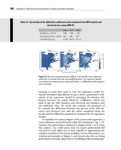
Table 5.2 Uncertainty of the diffusivity coefficients when estimated from QRS duration and
electrical axis, using LBM-EP.

c Myo c LV c RV
2
Total SD (σ T ,mm /s) 1482 1095 1191
2
Avg. bin-wise SD (σ i ,mm /s) 191 556 537
Uncertainty (σ i /σ T ) 12.9% 50.7% 45.1%

Figure 5.2. Bin-wise standard deviation (SD) in % of total SD of each diffusivity
coefficient, for known electrical axis and QRS duration. The regions of highest
uncertainty are clustered at the center of the plots, i.e. within the healthy range of
each parameter.

maining 18 cases were used to train the regression model. Us-
ing the simulated data allowed to get a direct, quantitative eval-
uation of the regression model by averaging the absolute dif-
ference between the actual diffusivity coefficients (which was
used to get the QRS duration and electrical axis features) and
the estimated ones. We could also evaluate the goodness of
fit, namely the difference between the ground truth QRS du-
ration and electrical axis, and the values computed using the
model and the diffusivity parameters estimated by the regression
model.
To establish the optimal degree of the polynomial regression, a
cross-validation was performed within the training set. Fig. 5.3 il-
lustrates the performance obtained at degrees from 1 to 8. From
this analysis, one could assess that low-degree polynomials did
not perform well, likely due to their inability to approximate the
solution manifold of the inverse problem. On the other hand, con-
sidering polynomials of degree 5 and beyond also did not bring
performance benefits, likely due to overfitting of the training sam-