Page 221 - Artificial Intelligence for Computational Modeling of the Heart

194 Chapter 6 Additional clinical applications

1. The points are expressed in Frenet coordinates with respect
to the centerline. For each point p on the surface, its corre-
sponding projection on the centerline p is found, and the
⊥
centerline normal n and bi-normal b vectors are computed at
point p . The surface point is transformed to the local coordi-
⊥
nate system as follows: p = (z,p · n,p · b) where z is the arc
F
length of the centerline segment given by the centerline start-
ing point and the projected point p .
⊥
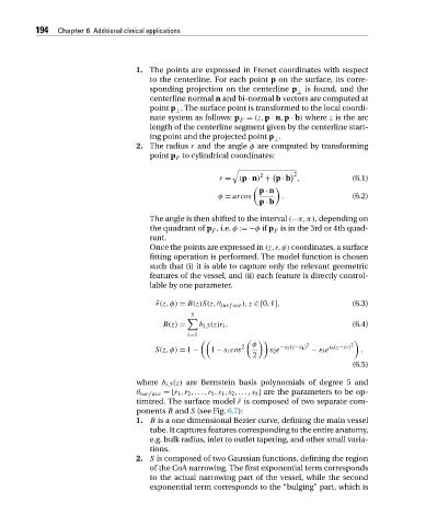
2. The radius r and the angle φ are computed by transforming
point p to cylindrical coordinates:
F
2
2
r = (p · n) + p · b , (6.1)
p · n

φ = arcos . (6.2)
p · b
The angle is then shifted to the interval (−π,π), depending on
the quadrant of p ,i.e. φ := −φ if p is in the 3rd or 4th quad-
F
F
rant.
Once the points are expressed in (z,r,φ) coordinates, a surface
fitting operation is performed. The model function is chosen
such that (i) it is able to capture only the relevant geometric
features of the vessel, and (ii) each feature is directly control-
lable by one parameter.
¯ r(z,φ) = B(z)S(z,θ surf ace ),z ∈[0,1], (6.3)
5

B(z) = b i,5 (z)r i , (6.4)
i=1

2 φ −s 3 (z−s 4 ) 2 s 6 (z−s 7 ) 2
S(z,φ) = 1 − 1 − s 1 cos s 2 e − s 5 e ,
2
(6.5)
where b i,5 (z) are Bernstein basis polynomials of degree 5 and
θ surf ace =[r 1 ,r 2 ,...,r 5 ,s 1 ,s 2 ,...,s 5 ] are the parameters to be op-
timized. The surface model ¯ is composed of two separate com-
r
ponents B and S (see Fig. 6.7):
1. B is a one dimensional Bezier curve, defining the main vessel
tube. It captures features corresponding to the entire anatomy,
e.g. bulk radius, inlet to outlet tapering, and other small varia-
tions.
2. S is composed of two Gaussian functions, defining the region
of the CoA narrowing. The first exponential term corresponds
to the actual narrowing part of the vessel, while the second
exponential term corresponds to the “bulging” part, which is