Page 354 - Automotive Engineering Powertrain Chassis System and Vehicle Body

Tyre characteristics and vehicle handling and stability C HAPTER 11.1

possible unstable motions that may show up with such ðm þ m c ÞY m c ðhj þ fqÞ
€
€
€
a combination. Linear differential equations are suffi- (11.1.109)
cient to analyse the stability of the straight ahead ¼ F y1 þ F y2 þ F y3
motion. We will again employ Lagrange’s equations to 2 € € €
ðI c þ m c f Þq m c fðY hjÞ¼ gF y3 (11.1.110)
set up the equations of motion. The original equations
2 €
€
€
(11.1.25) may be employed because the yaw angle is ðI þ m c h Þj m c hðY fqÞ
assumed to remain small. The generalised coordinates (11.1.111)
¼ aF y1 bF y2 hF y3
Y, j and q are used to describe the car’s lateral position
and the yaw angles of car and trailer, respectively. The This constitutes a system of the sixth order. By in-
forward speed dX/dt (z V z u) is considered to be troducing the velocities v and r the order can be reduced
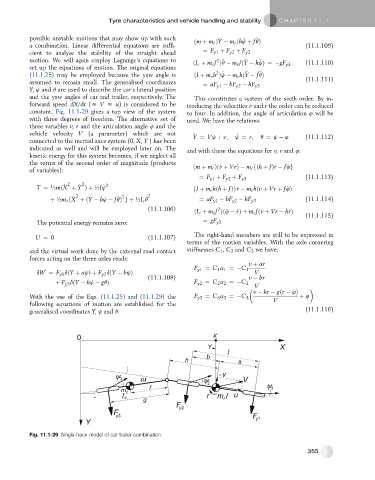
constant. Fig. 11.1-29 gives a top view of the system to four. In addition, the angle of articulation 4 will be
with three degrees of freedom. The alternative set of used. We have the relations:
three variables v, r and the articulation angle 4 and the
vehicle velocity V (a parameter) which are not _ j ¼ r; q ¼ j 4 (11.1.112)
_
connected to the inertial axes system (0, X, Y ) has been Y ¼ Vj þ v;
indicated as well and will be employed later on. The and with these the equations for v, r and 4:
kinetic energy for this system becomes, if we neglect all
the terms of the second order of magnitude (products ðm þ m c Þð_ v þ VrÞ m c fðh þ fÞ_ r f€ 4g
of variables):
¼ F y1 þ F y2 þ F y3 (11.1.113)
2
2
_
_ 2
_
T ¼ ½mðX þ Y Þþ ½Ij fI þ m c hðh þ fÞg_ r m c hð_ v þ Vr þ f€ 4Þ
2
_ 2
_
_
_
þ ½m c fX þðY hj fqÞ gþ ½I c q _ 2 ¼ aF y1 bF y2 hF y3 (11.1.114)
(11.1.106) ðI c þ m c f Þð€ 4 _ rÞþ m c fð_ v þ Vr h_ rÞ
2
(11.1.115)
The potential energy remains zero: ¼ gF y3
U ¼ 0 (11.1.107) The right-hand members are still to be expressed in
terms of the motion variables. With the axle cornering
and the virtual work done by the external road contact stiffnesses C 1 , C 2 and C 3 we have:
forces acting on the three axles reads:
v þ ar
F y1 ¼ C 1 a 1 ¼ C 1
dW ¼ F y1 dðY þ ajÞþ F y2 dðY bjÞ V
(11.1.108) v br
a
þ F y3 dðY hj gqÞ F y2 ¼ C 2 2 ¼ C 2
V
v hr gðr _ 4Þ
a
With the use of the Eqs. (11.1.25) and (11.1.29) the F y3 ¼ C 3 3 ¼ C 3 V þ 4
following equations of motion are established for the
generalised coordinates Y, j and q: (11.1.116)

Fig. 11.1-29 Single-track model of car trailer combination.

355