Page 351 - Automotive Engineering Powertrain Chassis System and Vehicle Body

CHAP TER 1 1. 1 Tyre characteristics and vehicle handling and stability

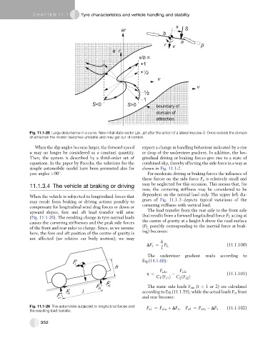
Fig. 11.1-25 Large disturbance in a curve. New initial state vector (Dv, Dr) after the action of a lateral impulse S. Once outside the domain
of attraction the motion becomes unstable and may get out of control.
When the slip angles become larger, the forward speed expect a change in handling behaviour indicated by a rise
u may no longer be considered as a constant quantity. or drop of the understeer gradient. In addition, the lon-
Then, the system is described by a third-order set of gitudinal driving or braking forces give rise to a state of
equations. In the paper by Pacejka, the solutions for the combined slip, thereby affecting the side force in a way as
simple automobile model have been presented also for shown in Fig. 11.1-2.

yaw angles >90 . For moderate driving or braking forces the influence of
these forces on the side force F y is relatively small and
11.1.3.4 The vehicle at braking or driving may be neglected for this occasion. This means that, for
now, the cornering stiffness may be considered to be
When the vehicle is subjected to longitudinal forces that dependent on the normal load only. The upper left dia-
may result from braking or driving actions possibly to gram of Fig. 11.1-3 depicts typical variations of the
compensate for longitudinal wind drag forces or down or cornering stiffness with vertical load.
upward slopes, fore and aft load transfer will arise The load transfer from the rear axle to the front axle
(Fig. 11.1-26). The resulting change in tyre normal loads that results from a forward longitudinal force F L acting at
causes the cornering stiffnesses and the peak side forces the centre of gravity at a height h above the road surface
of the front and rear axles to change. Since, as we assume (F L possibly corresponding to the inertial force at brak-
here, the fore and aft position of the centre of gravity is ing) becomes:
not affected (no relative car body motion), we may
h
DF z ¼ F L (11.1.100)
l
The understeer gradient reads according to
F Eq.(11.1.60):
L
h
F z1o F z2o
h ¼ (11.1.101)
C 1 ðF z1 Þ C 2 ðF z2 Þ
F
F x2 The static axle loads F zio (i ¼ 1 or 2) are calculated
z2
F l according to Eq.(11.1.59), while the actual loads F zi front
F x1
z1 and rear become:
Fig. 11.1-26 The automobile subjected to longitudinal forces and F z1 ¼ F z1o þ DF z ; F z2 ¼ F z2o DF z (11.1.102)
the resulting load transfer.

352