Page 346 - Automotive Engineering Powertrain Chassis System and Vehicle Body

Tyre characteristics and vehicle handling and stability C HAPTER 11.1

normalised characteristics at a given level of a y /g be-
comes now of importance. We define:
1 vF yi
F i ¼ ði ¼ 1; 2Þ (11.1.83)
F zi va i
The conditions for stability, that is: second and last
coefficient of equation comparable with Eq.(11.1.47)
must be positive, read after having introduced the radius
2
of gyration k (k ¼ I/m):

2
2
2
2
ðk þ a ÞF 1 þðk þ b ÞF 2 > 0 (11.1.84)

vd
F 1 F 2 > 0 (11.1.85)
v1=R V
The subscript V refers to the condition of differenti-
ation with V kept constant, that is while staying on the
speed line of Fig. 11.1-17. The first condition (11.1.84)
may be violated when we deal with tyre characteristics
showing a peak in side force and a downwards sloping
further part of the characteristic. The second condition
corresponds to condition (11.1.65) for the linear model.
Accordingly, instability is expected to occur beyond the
point where the steer angle reaches a maximum while
the speed is kept constant. This, obviously, can only occur
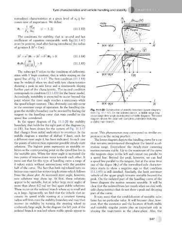
in the oversteer range of operation. In the handling dia-
gram the stability boundary can be assessed by finding the Fig. 11.1-20 Construction of stability boundary (upper diagram,
from Fig. 11.1-17). On the isolated branch, a stable range may
tangent to the handling curve that runs parallel to the
occur (large steer angle as indicated in middle diagram). The lower
speed line considered. diagram shows the case with complete understeer featuring
In the upper diagram of Fig. 11.1-20 the stability a stable main branch.
boundary, that holds for the right part of the diagram (a y
vs l/R), has been drawn for the system of Fig. 11.1-17
that changes from initial understeer to oversteer. In the occur. This phenomenon may correspond to similar ex-
middle diagram a number of shifted V-lines, each for periences in the racing practice.
a different steer angle d, has been indicated. In each case The lower diagram depicts the handling curve for a car
the points of intersection represent possible steady-state that remains understeered throughout the lateral accel-
solutions. The highest point represents an unstable so- eration range. Everywhere the steady-state cornering
lution as the corresponding point on the speed line lies in motion remains stable. Up to the maximum of the curve
the unstable area. When the steer angle is increased the the tangents slope to the left and cannot run parallel to
two points of intersections move towards each other. It a speed line. Beyond the peak, however, we can find
turns out that for this type of handling curve a range of a speed line parallel to the tangent, but at the same time
d values exists without intersections with the positive one of the slopes (F 1 ) of the normalised axle character-
half of the curve. The fact that both right-hand turn so- istics starts to show a negative sign so that condition
lutions may vanish has serious implications which follows (11.1.85) is still satisfied. Similarly, the limit oversteer
from the phase plot. At increased steer angle, however, vehicle of the upper graph remains unstable beyond the
new solutions may show up. At first, these solutions peak. On the isolated part of the handling curve of the
appear to be unstable, but at rather large steer angles of lower diagram the motion remains unstable. It will be
more than about 0.2 rad we find again stable solutions. clear that the isolated branches vanish when we deal with
These occur on the isolated branch where a 2 is small and axle characteristics that do not show a peak and decaying
a 1 is large. Apparently, we find that the vehicle that in- part of the curve.
creases its speed while running at a constant turning It may seem that the establishment of unstable solu-
radius will first cross the stability boundary and may then tions has no particular value. It will become clear, how-
recover its stability by turning the steering wheel to ever, that the existence and the location of both stable
a relatively large angle. In the diagram the left part of the and unstable singular points play an important role in
isolated branch is reached where stable spirals appear to shaping the trajectories in the phase-plane. Also, the

347