Page 341 - Automotive Engineering Powertrain Chassis System and Vehicle Body

CHAP TER 1 1. 1 Tyre characteristics and vehicle handling and stability

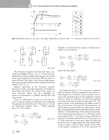
Fig. 11.1-14 Step response of yaw rate to steer angle. Parameters according to Table 11.1-1. Parameter influence on the rise time t r .

0 1 0 1
C Cs C 1
V þ Similarly, the formula for the response of lateral accel-
B mV mV C B m C eration a y can be derived:
C
A ¼ B 2 A ; B ¼ B C
@
@
A
Cs Cq C 1 a
2
2
mk V mk V mk 2 mk 2 2 b
0 1 0 1 a y a y 1 C 2 l u þ V ju
C Cs C 1 ðjuÞ¼ , ;
u 2
B mV mV C B m C d d ss 1 u o þ 2z ju
B
B
u o
C;
C ¼ B C D ¼ B C 2 (11.1.78)
C
@ 0 1 A @ 0 A a y V =l
¼ h
1=V 0 0 d ss 1 þ V 2
gl
(11.1.76)
and for the slip angle b:
The frequency response functions have been com-
puted using Matlab software. Fig. 11.1-15 presents the
2
mk V
amplitude and phase response functions for each of the b 1 amV bC 2 l ju
b
2
three output quantities and at three different values of d ðjuÞ¼ d , ;
u 2
ju
speed of travel. The values of the chosen model param- ss 1 u o þ2z u o (11.1.79)
eters and a number of characteristic quantities have been b 1 a m V 2
b
b C 2 l
listed in Table 11.1-1. d ¼ l h 2
Explicit expressions of the frequency response ss 1 þ gl V
functions in terms of model parameters are helpful to
understand and predict the characteristic aspects of By considering Eq.(11.1.77) it can now be explained
these functions which may be established by that for instance at higher frequencies the system ex-
means of computations or possibly through full scale hibits features of a first-order system: because of the ju
experiments. term in the numerator the yaw rate amplitude response
From the differential equation (11.1.50) the fre- tends to a decay at a 6 dB per octave rate (when plotted

quency response function is easily derived. Considering in log–log scale) and the phase lag approaches 90 . The
phase increase at low frequencies and higher speeds is
the quantities formulated by (11.1.70) and (11.1.71) and
due to the presence of the speed V in that same term. At
the steady-state response (r/d) ss ¼ (V/R)/d obtained
speeds beyond approximately the characteristic speed,
from (11.1.56) we find:
the corresponding (last) term in the denominator has less
influence on the initial slope of the phase characteristic.
mVa
r r 1 þ C 2 l ju The lateral acceleration response (11.1.78) shown in the
ðjuÞ¼ , ; centre graph of Fig. 11.1-15 gives a finite amplitude at
d d ss 1 u 2 þ 2z ju
u o u o frequencies tending to infinity because of the presence of
(11.1.77) 2
r V=l u in the numerator. For the same reason, the phase lag
¼ h
d ss 1 þ V 2 goes back to zero at large frequencies. The side slip phase
gl response tends to –270 (at larger speeds) which is due

to the negative coefficient of ju in the numerator of
342