Page 343 - Automotive Engineering Powertrain Chassis System and Vehicle Body

CHAP TER 1 1. 1 Tyre characteristics and vehicle handling and stability

Table 11.1-1 Parameter values and typifying quantities

Parameters Derived typifying quantities
a 1.4 m l 3m V [m/s] 20 40 60
b 1.6 m F z1 8371 N u o [rad/s] 4.17 2.6 2.21

C 1 60000 N/rad F z2 7325 N z [–] 0.9 0.7 0.57
60000 N/rad q 1.503 m u n [rad/s] 1.8 1.8 1.82
C 2
m 1600 kg s 0.1 m t r [s] 0.23 0.3 0.27

k 1.5 m h 0.0174 rad (w1 extra steer/g lateral accel.)

equal to zero. In practice, this may be done to improve where K ¼ ma y represents the centrifugal force. The
handling qualities of the automobile (reduces to first- kinematic relationship
order system!) and to avoid excessive side slipping
motions of the rear axle in lane change manoeuvres. l
Adapt the equations of motion (11.1.46) and assess d ða 1 a Þ¼ (11.1.81)
2
the required relationship between the steer angles d 1 R
and d 2 . Do this in terms of the transfer function be- follows from Eqs.(11.1.44) and (11.1.51). In Fig. 11.1-11
tween d 2 and d 1 and the associated differential equa- the vehicle model has been depicted in a steady-state
tion. Find the steady-state ratio (d 2 /d 1 ) ss and plot this cornering manoeuvre. It can easily be observed from this
as a function of the speed V. Show also the frequency diagram that relation (11.1.81) holds approximately
response function d 2 /d 1 (ju) for the amplitude and when the angles are small.
phase at a speed V ¼ 30 m/s. Use the vehicle param- The ratio of the side force and vertical load as shown
eters supplied in Table 11.1-1.
in (11.1.80) plotted as a function of the slip angle may be
termed as the normalised tyre or axle characteristic.
11.1.3.3 Non-linear steady-state These characteristics subtracted horizontally from each
cornering solutions other produce the ‘handling curve’. Considering the equal-
ities (11.1.80)the ordinate maybereplacedby a y /g.The
From Eqs.(11.1.42) and (11.1.59) with the same re- resulting diagram with abscissa a 1 a is the non-linear
2
strictions as stated below Eq.(11.1.60), the following version of the right-hand diagram of Fig. 11.1-10 (rotated

force balance equations can be derived (follows also from 90 anti-clockwise). The diagram may be completed by
Eqs.(11.1.61)) (the effect of the pneumatic trails will be attaching the graph that shows for a series of speeds V
dealt with later on): the relationship between lateral acceleration (in g units)
a y /g and the relative path curvature l/R according to

F y1 F y2 a y K Eq.(11.1.55).
¼ ¼ ¼ (11.1.80)
F z1 F z2 g mg Fig. 11.1-17 shows the normalised axle characteristics
and the completed handling diagram. The handling curve
l consists of a main branch and two side lobes. The dif-
b ferent portions of the curves have been coded to indicate
a the corresponding parts of the original normalised axle
characteristics they originate from. Near the origin the
2 -v system may be approximated by a linear model. Conse-
V quently, the slope of the handling curve in the origin with
1 respect to the vertical axis is equal to the under steer co-
r u efficient h. In contrast to the straight handling line of the
F 2
y2 1 linear system (Fig. 11.1-10), the non-linear system shows
a curved line. The slope changes along the curve which
F means that the degree of understeer changes with in-
y1
creasing lateral acceleration. The diagram of Fig. 11.1-17
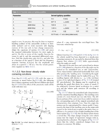
Fig. 11.1-16 ‘Four-wheel’ steering to make slip angle b ¼ 0 shows that the vehicle considered changes from un-
(Exercise 11.1.2). dersteer to oversteer. We define:

344