Page 338 - Automotive Engineering Powertrain Chassis System and Vehicle Body

Tyre characteristics and vehicle handling and stability C HAPTER 11.1

and fore and aft load transfer at braking or driving should
not be introduced in expression (11.1.60).
In the same diagram the difference in slip angle front
and rear may be indicated. We find for the side forces:

b a y a a y
F y1 ¼ ma y ¼ F z1 ; F y2 ¼ ma y ¼ F z2
l g l g
(11.1.61)

and hence for the slip angles:

F z1 a y F z2 a y
a 1 ¼ ; a ¼ (11.1.62)
2
C 1 g C 2 g
The difference now reads when considering the
relation (11.1.59) as:

a y
a 1 a ¼ h (11.1.63)
2
g
Apparently, the sign of this difference is dictated by
the understeer coefficient. Consequently, it may be
stated that according to the linear model an understeered
vehicle (h > 0) moves in a curve with slip angles larger at
the front than at the rear (a 1 > a 2 ). For a neutrally
steered vehicle the angles remain the same (a 1 ¼a 2 ) and Fig. 11.1-11 Two-wheel vehicle model in a cornering manoeuvre.
with an oversteered car the rear slip angles are bigger
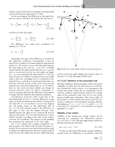
(a 2 > a 1 ). As is shown by the expressions (11.1.54), the and the vehicle slip angle changes into positive values. In
signs of h and s are different. Consequently, as one might Exercise 11.1.2 the slip angle b will be used.
expect when the centrifugal force is considered as the
external force, a vehicle acts oversteered when the neu- 11.1.3.2.2 Influence of the pneumatic trail
tral steer point lies in front of the centre of gravity and The direct influence of the pneumatic trails t i may not be
understeered when S lies behind the c.g.. As we will see negligible. In reality, the tyre side forces act a small dis-
later on, the actual non-linear vehicle may change its tance behind the contact centres. As a consequence, the
steering character when the lateral acceleration in- neutral steer point should also be considered to be lo-
creases. It appears then that the difference in slip angle is cated at a distance approximately equal to the average
no longer directly related to the understeer gradient. value of the pneumatic trails, more to the rear, which
Consideration of Eq.(11.1.56) reveals that in the means actually more understeer. The correct values of
left-hand graph of Fig. 11.1-10 thedifferenceinslip the position s of the neutral steer point and of the un-
angle can be measured along the ordinate starting from dersteer coefficient h can be found by using the effective
0
the value l/R. It is of interest to convert the diagram axle distances a ¼ a t 1 ; b ¼ b þ t 2 and l ¼ a þ b 0
0
0
0
into the graph shown on the right-hand side of in the Eqs.(11.1.48) and (11.1.59) instead of the original
Fig. 11.1-10 with ordinate equal to the difference in quantities a, b and l.
slip angle. In that way, the diagram becomes more
flexible because the value of the curvature l/R may be Stability of the motion
selected afterwards. The horizontal dotted line is then Stability of the steady-state circular motion can be
shifted vertically according to the value of the relative
curvature l/R considered. The distance to the handling examined by considering the differential equation
line represents the magnitude of the steer angle. (11.1.47) or (11.1.50). The steer angle is kept constant so
Fig. 11.1-11 depicts the resulting steady-state cor- that the equation gets the form:
nering motion. The vehicle side slip angle b has been in- a 0 r þ a 1 _ r þ a 2 r ¼ b 1 d (11.1.64)
€
dicated. It is of interest to note that at low speed this angle
is negative for right-hand turns. Beyond a certain value of For this second-order differential equation stability is
speed the tyre slip angles have become sufficiently large assured when all coefficients a i are positive. Only the

339