Page 333 - Automotive Engineering Powertrain Chassis System and Vehicle Body

CHAP TER 1 1. 1 Tyre characteristics and vehicle handling and stability

X
F
l y1
Y b
a M
M z1
z2 -v
V 1
2 F =0
x2
1
F x2
r u x F
y2
F M z1
y2
F
y F y1 x2
2
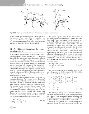
Fig. 11.1-9 Simple car model with side force characteristics for front and rear (driven) axle.

force F x on the tyre or axle cornering force vs slip angle The system depicted in Fig. 11.1-4 and described in
characteristic (F y , a) may then be regarded (cf. the preceding subsection performs a motion over a flat
Fig. 11.1-9). The forces F y1 and F x1 and the moment level road. Proper coordinates are the Cartesian co-
M z1 are defined to act upon the single front wheel and ordinates X and Yof reference point A, the yaw angle j of
similarly we define F y2 etc. for the rear wheel. the moving x axis with respect to the inertial X axis and
finally the roll angle 4 about the roll axis. For motions
near the X axis and thus small yaw angles, Eq.(11.1.25)is
11.1.3.1 Differential equations for plane adequate to derive the equations of motion. For cases
vehicle motions where j may attain large values, e.g. when moving along
a circular path, it is preferred to use modified equations
In this section, the differential equations for the three- where the velocities u, v and r of the moving axes system
degree-of-freedom vehicle model of Fig. 11.1-4 will be are used as generalised motion variables in addition to the
derived. In first instance, the fore and aft motion will also coordinate 4. The relations between the two sets of
be left free to vary. The resulting set of equations of variables are (the dots referring to differentiation with
motion may be of interest for the reader to further study respect to time):
_
_
the vehicle’s dynamic response at somewhat higher fre- u ¼ X cos j þ Y sin j
_
_
quencies where the roll dynamics of the vehicle body v ¼ X sin j þ Y cos j (11.1.26)
_
may become of importance. From these equations, the r ¼ j
equations for the simple two-degree-of-freedom model
of Fig. 11.1-9 used in the subsequent section can be easily The kinetic energy can be expressed in terms of u, v
assessed. In Subsection 11.1.3.6 the equations for the car and r. Preparation of the first terms of Eq.(11.1.25) for
with trailer will be established. The possible instability of the coordinates X, Y and j yields:
the motion will be studied. vT vT vu vT vv vT vT
We will employ Lagrange’s equations to derive the ¼ þ ¼ cos j sin j
_
_
_
equations of motion. For a system with n degrees of vX vu vX vv vX vu vv
freedom n (generalised) coordinates q i are selected vT ¼ vT vu þ vT vv ¼ vT sin j þ vT cos j
_
_
_
which are sufficient to completely describe the motion vY vu vY vv vY vu vv
while possible kinematic constraints remain satisfied. vT ¼ vT
The moving system possesses kinetic energy T and vj _ vr
potential energy U. External generalised forces Q i asso- vT vT vT
ciated with the generalised coordinates q i may act on the vj ¼ vu v vv u (11.1.27)
system and do work W. Internal forces acting from
dampers to the system structure may be regarded The yaw angle j may now be eliminated by multi-
as external forces taking part in the total work W. plying the final equations for X and Y successively with
The equation of Lagrange for coordinate q i reads: cos j and sin j and subsequently adding and subtracting
them. The resulting equations represent the equilibrium
d vT vT vU in the x and y (or u and v) directions, respectively.
þ ¼ Q i (11.1.25)
dt v_ q i vq i vq i We obtain the following set of modified Lagrangean
equations for the first three variables u, v and r and

334