Page 347 - Automotive Engineering Powertrain Chassis System and Vehicle Body

CHAP TER 1 1. 1 Tyre characteristics and vehicle handling and stability

nature of stability or instability in the singular points are 4. The stability boundary (associated with these
of importance. oversteer ranges) in the (a y /g vs l/R) diagram
(¼ right-hand side of the handling diagram)
Exercise 11.1.3. Construction of the complete (cf. Fig. 11.1-20).
handling diagram from pairs of axle 5. Indicate in the diagram (or in a separate graph):
characteristics
a. the course of the steer angle d required to negoti-
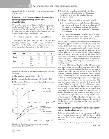
We consider three sets of hypothetical axle characteris- ate a curve with radius R ¼ 60 m as a function of
tics (a, b and c) shown in the graph of Fig. 11.1-21. The the speed V. If applicable, indicate the stability
dimensions of the vehicle model are: a ¼ b ¼ ½l ¼ 1.5 m. boundary, that is the critical speed V crit , belonging
For the tyres we may employ axle characteristics de- to this radius.
scribed by the Magic Formula (11.1.6):
b. the course of steer angle d as a function of relative
F y ¼ D sin½C arctanfBa EðBa arctanðBaÞÞgŠ path curvature l/R at a fixed speed V ¼ 72 km/h
and if applicable assess the critical radius R crit .
We define: the peak side force D ¼ mF z and the For the vehicle systems considered so far a unique han-
cornering stiffness C Fa ¼ BCD ¼ C Fa F z so that B ¼ dling curve appears to suffice to describe the steady-state
C Fa /(Cm). For the six tyre/axle configurations the para- turning behaviour. Cases may occur, however, where
meter values have been given in the table below.
more curves are needed, one for each velocity. A simple
example is the situation when the car runs over a wet
surface where the tyre characteristics change consider-
Axle Case m C Fa C E ably with speed. Also, as a result of the down forces

Front a,b 0.8 8 1.2 –2 acting on e.g. the body of a racing car, the tyre loads in-
c 0.78 8 1.3 –2 crease with speed. Consequently, the tyre characteristics
Rear a 0.9 11 1.2 –2 change accordingly which requires an adaptation of the
b 0.9 6 1.2 –2 handling curve.
c 0.65 11 1.5 1 A more difficult and fundamentally different situa-
tion occurs when the vehicle is equipped with a third
axle. Also in this case multiple handling curves arise. A
Determine for each of the three combinations (two dry, tandem rear axle configuration of a heavy truck for
one wet): example, strongly opposes movement along a curved
1. The handling curve (cf. Fig. 11.1-17). track. The slip angles of the two rear axles are different
so that a counteracting torque arises. This torque gets
2. The complete handling diagram (cf. Fig. 11.1-17).
larger when the turning radius becomes smaller. This
3. The portion of the curves where the vehicle shows an may for instance occur at a given level of lateral accel-
oversteer nature. eration. When at this level the speed becomes lower,
the curvature must become larger and the opposing
torque will increase which entails an increased front
steer angle to generate a larger side force needed to
balance the vehicle. This increased steer angle goes on
top of the steer angle which was already larger because
of the increased l/R. Here, l is the average wheel base.
Consequently, in the handling diagram, the points on
the handling curve belonging to the lower speed lie
more to the left.

Assessment of the influence of the pneumatic
trail on the handling curve
So far the direct influence of the pneumatic trails have
not been taken into account. As with the linear analysis
we may do this by considering the effective axle
positions

0 0 0 0 0
a ¼ a t 1 ; b ¼ b þ t 2 and l ¼ a þ b
Fig. 11.1-21 Three sets of hypothetical axle cornering
characteristics (Exercise 11.1.3). (11.1.86)

348