Page 172 - Autonomous Mobile Robots

156 Autonomous Mobile Robots

Y b 2 b 1
b 2
b 1
b 3
y l u
b 6

b
b 4 5
x l X

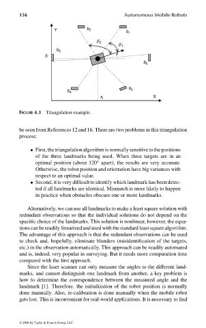
FIGURE 4.3 Triangulation example.

be seen from References 12 and 16. There are two problems in this triangulation
process:

• First, thetriangulationalgorithmisnormallysensitivetothepositions
of the three landmarks being used. When three targets are in an
optimal position (about 120 apart), the results are very accurate.
◦
Otherwise, the robot position and orientation have big variances with
respect to an optimal value.
• Second, it is very difficult to identify which landmark has been detec-
ted if all landmarks are identical. Mismatch is more likely to happen
in practice when obstacles obscure one or more landmarks.

Alternatively, we can use all landmarks to make a least square solution with
redundant observations so that the individual solutions do not depend on the
specific choice of the landmarks. This solution is nonlinear, however, the equa-
tions can be readily linearized and used with the standard least square algorithm.
The advantage of this approach is that the redundant observations can be used
to check and, hopefully, eliminate blunders (misidentification of the targets,
etc.) in the observation automatically. This approach can be readily automated
and is, indeed, very popular in surveying. But it needs more computation time
compared with the first approach.
Since the laser scanner can only measure the angles to the different land-
marks, and cannot distinguish one landmark from another, a key problem is
how to determine the correspondence between the measured angle and the
landmark [1]. Therefore, the initialization of the robot position is normally
done manually. Also, re-calibration is done manually when the mobile robot
gets lost. This is inconvenient for real-world applications. It is necessary to find

© 2006 by Taylor & Francis Group, LLC

FRANKL: “dk6033_c004” — 2006/3/31 — 16:42 — page 156 — #8