Page 34 - Autonomous Mobile Robots

Visual Guidance for Autonomous Vehicles 17

Model update mechanism. As the vehicle moves, new sensed data inputs can
either replace the historical ones, or a map-updating algorithm can be activated.
We will see real examples of occupancy grids in Section 1.5.3 and
Section 1.3.6 (Figure 1.8 and Figure 1.9).

1.3.3 Physical Limitations

We now examine the performance criteria for visual perception hardware with
regards to the classes of UGVs. Before we even consider algorithms, the phys-
ical realities of the sensing tasks are quite daunting. The implications must
be understood and we will demonstrate with a simple analysis. A wide FOV
is desirable so that there is a view of the road in front of the vehicle at close
range. The combination of lens focal length (f ) and image sensor dimensions
(H, V) determine the FOV and resolution. For example, a 1/2" sensor has image
dimensions (H = 6.4 mm, V = 4.8 mm). The angle of view (horizontally) is
approximated by
H
θ H = 2 arctan (1.6)
2f

and it is easily calculated that a focal length of 5 mm will equate to an angle
◦
of view of approximately 65 with a sensor of this size. It is also useful to
quote a value for the angular resolution; for example, the number of pixels per
degree. With an output of 640 × 480 pixels, the resolution for this example is
approximately 10 pixels per degree (or 1.75 mrad/pixel).
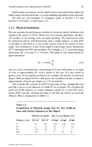
Now consider the scenario of a UGV progressing along a straight flat road
and that it has to avoid obstacles of width 0.5 m or greater. We calculate the
pixel size of the obstacle, at various distances ahead, for a wide FOV and a
narrow FOV, and also calculate the time it will take the vehicle to reach the
obstacle. This is summarized in Table 1.2.

TABLE 1.2
Comparison of Obstacle Image Size for Two Fields-of-
View and Various Distances to the Object

Obstacle size (pixel) Time to cover distance (sec)
Distance, d (m) FOV 60 ◦ FOV 10 ◦ 120 kph 60 kph 20 kph
8 35 113 0.24 0.48 1.44
20 14 45 0.6 1.2 3.6
50 5.6 18 1.5 3 9
300 0.9 3 9 18 54

© 2006 by Taylor & Francis Group, LLC

FRANKL: “dk6033_c001” — 2006/3/31 — 16:42 — page 17 — #17