
Page 39 - Autonomous Mobile Robots
P. 39
22 Autonomous Mobile Robots
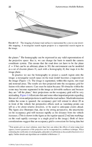
FIGURE 1.5 The imaging of planar road surface is represented by a one-to-one invert-
ible mapping. A rectangular search region projects to a trapezoidal search region in
the image.
3
the planes. The homography can be expressed in any valid representation of
the projective space: that is, we can change the basis to match the camera
coordinate system. This means that the road does not have to be the plane
Z = 0 but can be an arbitrary plane in 3D; the environment can be modeled
as a set of discrete planes i each with a homography H i that maps it to the
image plane.
In practice we use the homography to project a search region onto the
image; a rectangular search space on the road model becomes a trapezoid on
the image (Figure 1.5). The image is segmented, within this region, into road
and nonroad areas. The results are then projected onto the occupancy grid for
fusion with other sensors. Care must be taken because 3D obstacles within the
scene may become segmented in the image as driveable surfaces and because
they are “off the plane,” their projections on the occupancy grid will be very
misleading. Figure 1.6 illustrates this and some other important points regarding
this use ofvision and projectionsto and from the road surface. Much information
within the scene is ignored; the occupancy gird will extend to about 20 m
in front of the vehicle but perspective effects such as vanishing points can
tell us a lot about relative direction, or be used to anticipate events ahead.
The figure also illustrates that, due to the strong perspective, the uncertainty
on the occupancy grid will increase rapidly as the distance from the vehicle
increases. (This is shown in the figure as the regular spaced [2 m] lane markings
on the road rapidly converge to a single pixel in the image.) Both of these
considerations suggest that an occupancy grid is convenient for fusing data but
3 Four points give an exact solution; more than four can reduce the effects of noise using least
squares; known parameters of the projection can be incorporated in a nonlinear technique. When
estimating the coefficients of a homography, principles of calibration as discussed in Section 4.2.2.2
apply. Further details and algorithms are available in Reference 13.
© 2006 by Taylor & Francis Group, LLC
FRANKL: “dk6033_c001” — 2006/3/31 — 16:42 — page 22 — #22