Page 118 - Basic Structured Grid Generation

Structured grid generation – algebraic methods 107

E
D

Chord
F A B C

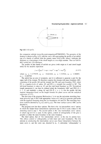
Fig. 4.22 Airfoil profile.

the companion website (www.bh.com/companions/0750650583). The geometry of the
domain is shown in Fig. 4.22, with the curve AB representing the profile of an airfoil,
one of a family of airfoils with the generic name NACA-00t, where t indicates the
thickness as a percentage of the chord length as a two-digit number. Thus an NACA-
0012 airfoil has 12% thickness.
The profiles of this family of airfoils are given (with origin at A and chord length
unity) by the analytic expression

1 2 3 4
y = t a 1 x 2 + a 2 x + a 3 x + a 4 x + a 5 x , (4.117)
where a 1 = 1.4779155, a 2 =−0.624424, a 3 = 1.727016, a 4 = 1.384087,
a 5 =−0.489769.
The airfoil has an axis of symmetry, and it is sufficient to generate a grid for the
upper half of the domain. We therefore consider the domain with inner boundary ABC,
consisting of the profile AB and the straight line CD, and outer boundary FED, where
FE is a quarter-circle of radius AE and ED is a straight line parallel to BC. The
left-hand boundary is taken as AF and the right-hand boundary as CD. Normalized
length parameters ξ can then be defined along the boundaries ABC and FED (0
ξ 1), and similarly η along AF and CD (0 η 1). For the profile AB this
requires integration based on the length formula for plane curves and the analytical
expression (4.117).
The first step of the program Multisurface.f is to use the univariate stretching func-
tions given by eqn (4.103) with appropriate values of P and Q to generate grid-nodes
with the required clustering along the two boundaries AF and CD. The stretching func-
tions could be denoted by h AF (η) and h CD (η). The inner surface (curve) ABC can be
denoted r 1 .
The program now has three options. The first is the ‘no intermediate curve’ option,
in which the simple linear interpolation expression eqn (4.116) is used, subject to the
stretching used in step 1. The second option is the ‘one intermediate curve’ option,
in which eqn (4.112) is used. In this option, control of orthogonality of the grid is
possible at either the inner boundary or the outer boundary.
The third option, that of ‘two intermediate curves’, is the one we pursue here.
This allows control of orthogonality at both inner and outer boundaries. The first
attempt at constructing the intermediate curves uses linear interpolation between the
inner curve r 1 and the outer one, denoted by r 4 . A subroutine ‘orthogonality’ is