Page 114 - Basic Structured Grid Generation

Structured grid generation – algebraic methods 103

which cluster grids near any number of stipulated lines. For example, clustering near
the two lines y = y 1 and y = y 2 is achieved by the combination

 1 [h − f(1 − η/η 1 )], 0 η η 1
η


hη 1 + (η 0 − η 1 )f ((η − η 1 )/(η 0 − η 1 )), η 1 η η 0

y = (4.101)
hη 0 + (η 2 − η 0 )[h − f ((η 2 − η)/(η 2 − η 0 ))],η 0 η η 2


hη 2 + (1 − η 2 )f ((η − η 2 )/(1 − η 2 )), η 2 η 1.
where f(η) is again given by eqn (4.93), y = y 0 is any value intermediate to y 1 and
y 2 ,and η j = y j /h, j = 0, 1, 2. Thus we have, explicitly,
 α α(1−η/η 1 ) α
hη 1 [e − e ]/(e − 1), 0 η η 1

hη 1 + (η 0 − η 1 )h(e − 1)/(e − 1), η 1 η η 0
 α(η−η 1 )/(η 0 −η 1 ) α

y = (4.102)
α
hη 2 − (η 2 − η 0 )h(e α(η 2 −η)/(η 2 −η 0 ) − 1)/(e − 1), η 0 η η 2


 α(η−η 2 )/(1−η 2 ) α
hη 2 + (1 − η 2 )h(e − 1)/(e − 1), η 2 η 1.
Similar expressions can be formulated on the basis of the stretching functions defined
in eqns (4.88) and (4.92), and similar monotonically increasing functions can be defined
to locate grid clustering near an arbitrary number of lines y = const..
4.5 Two-boundary and multisurface methods
4.5.1 Two-boundary technique

The example of the divergent nozzle in the previous section shows how a two-
dimensional grid can be generated in the physical domain between two boundaries,
using stretching functions to control grid-density. The techniques described here start
from these basic ideas, and incorporate Hermite interpolation to produce orthogonality
at the boundaries. Moreover, stretching functions are used along the curved boundaries
to produce the required position of grid-nodes.
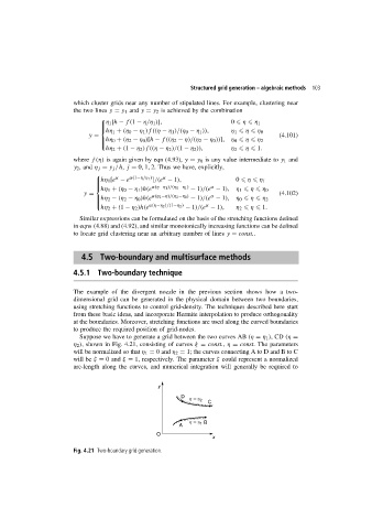
Suppose we have to generate a grid between the two curves AB (η = η 1 ),CD (η =
η 2 ), shown in Fig. 4.21, consisting of curves ξ = const., η = const. The parameters
will be normalized so that η 1 = 0and η 2 = 1; the curves connecting A to D and B to C
will be ξ = 0and ξ = 1, respectively. The parameter ξ could represent a normalized
arc-length along the curves, and numerical integration will generally be required to

y
D
h = h 2
C

h = h 1 B
A
O
x
Fig. 4.21 Two-boundary grid generation.