Page 110 - Basic Structured Grid Generation

Structured grid generation – algebraic methods 99

y h
h
1

0 0
L x 1 x

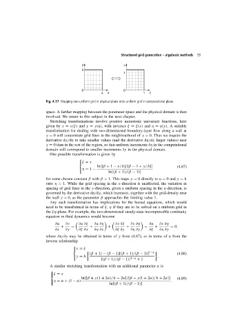
Fig. 4.17 Mapping non-uniform grid in physical plane onto uniform grid in computational plane.

space. A further mapping between the parameter space and the physical domain is then
involved. We return to this subject in the next chapter.
Stretching transformations involve positive monotonic univariate functions, here
given by x = x(ξ) and y = y(η), with inverses ξ = ξ(x) and η = η(y). A suitable
transformation for dealing with two-dimensional boundary-layer flow along a wall at
y = 0 will concentrate grid lines in the neighbourhood of y = 0. Thus we require the
derivative dy/dη to take smaller values (and the derivative dη/dy larger values) near
y = 0 than in the rest of the region, so that uniform increments δη in the computational
domain will correspond to smaller increments δy in the physical domain.
One possible transformation is given by


ξ = x
ln{[β + 1 − y/h]/[β − 1 + y/h]} (4.87)
η = 1 −
ln{(β + 1)/(β − 1)}
for some chosen constant β with β> 1. This maps y = 0 directly to η = 0and y = h
onto η = 1. While the grid spacing in the x-direction is unaffected, the variation in
spacing of grid lines in the y-direction, given a uniform spacing in the η-direction, is
governed by the derivative dη/dy, which increases, together with the grid-density near
the wall y = 0, as the parameter β approaches the limiting value 1.
Any such transformation has implications for the hosted equations, which would
need to be transformed in terms of ξ, η if they are to be solved on a uniform grid in
the ξη-plane. For example, the two-dimensional steady-state incompressible continuity
equation in fluid dynamics would become

∂u ∂v ∂u ∂ξ ∂u ∂η ∂v ∂ξ ∂v ∂η ∂u ∂v ∂η
+ = + + + = + = 0,
∂x ∂y ∂ξ ∂x ∂η ∂x ∂ξ ∂y ∂η ∂y ∂ξ ∂η ∂y
where ∂η/∂y may be obtained in terms of y from (4.87), or in terms of η from the
inverse relationship

x = ξ
1−η
(β + 1) − (β − 1)[(β + 1)/(β − 1)] (4.88)
y = h .
[(β + 1)/(β − 1)] 1−η + 1
A similar stretching transformation with an additional parameter α is

ξ = x
ln{[β + y(1 + 2α)/h − 2α]/[β − y(1 + 2α)/h + 2α]} (4.89)
η = α + (1 − α) .
ln[(β + 1)/(β − 1)]