Page 107 - Basic Structured Grid Generation

96 Basic Structured Grid Generation

A complete program may be found on the accompanying disk as described in
Section 4.6.4.

4.3.3 Three-dimensional TFI

A simple approach to TFI in three dimensions is through the extension of the definition
of projectors to 3D. Suppose that we have a mapping r(ξ, η, ς) from the unit cube
0 ξ 1, 0 η 1, 0 ς 1 to a six-sided volume R of physical space.
The opposite planar faces of the cube given by ξ = 0, 1 map onto the (in general,
curved) opposite faces r(0,η, ς), r(1,η, ς) of R. On these faces there are curvilinear
co-ordinate systems with η and ς as co-ordinates. Edges of the cube such as that given
by η = ς = 0 (with 0 ξ 1) map into edges of R such as r(ξ, 0, 0),which is a
ξ-co-ordinate curve.
Using linear Lagrange polynomials as blending functions, the following projectors
may be defined:

P ξ (ξ,η,ς) = (1 − ξ)r(0,η, ς) + ξr(1,η,ς) (4.78)
P η (ξ,η,ς) = (1 − η)r(ξ, 0,ς) + ηr(ξ, 1,ς) (4.79)

P ς (ξ,η,ς) = (1 − ς)r(ξ, η, 0) + ςr(ξ, η, 1). (4.80)

Now the projector P ξ still maps the opposite faces ξ = 0, 1 of the cube onto the
opposite faces r(0,η,ς), r(1,η,ς) of R. It also maps all the vertices of the cube,
(0, 0, 0), (1, 0, 0), etc., onto the vertices r(0, 0, 0), r(1, 0, 0),etc., of R. However, the
four edges of the cube which connect opposite vertices of the faces ξ = 0and ξ = 1
are mapped onto straight lines connecting corresponding vertices of R.
For example, (ξ, 0, 0) → (1 − ξ)r(0, 0, 0) + ξr(1, 0, 0),0 ξ 1.
Clearly the other projectors P η , P ς have similar properties. Moreover they all satisfy
the basic projection property given by eqn (4.71).
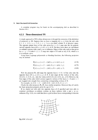
If we started out with only two opposite faces of R specified and were able to
construct curvilinear co-ordinate systems on these surfaces with η and ς as co-
ordinates (Fig. 4.16), we could then have a grid on these faces corresponding to discrete

h = 1

= 1
= 0

h = 0

Fig. 4.16 Surface grid.