Page 103 - Basic Structured Grid Generation

92 Basic Structured Grid Generation

In all the above approaches a matrix equation has to be solved for the values of

y , y ,...,y . The matrix A is tridiagonal and diagonally dominant in each case,
1 2 n−1
and possesses a large degree of sparseness. There are standard numerical methods of
solving such a system, such as the Thomas Algorithm (see Section 5.2). It is then
straightforward to calculate y and y , and we are then in a position to calculate the

0 n
interpolating cubic spline itself from eqn (4.50).
The same remarks hold for the following.
Method 5 Here we may consider a mixture of end-conditions of the type considered
in the previous four approaches. For example, one might have a natural spline at the
left-hand end (Method 1) with a specified slope at the right-hand end (Method 3). In
this case we simply have to take the matrix A as in eqn (4.54) but change the last row
in accordance with eqn (4.66). Moreover, the column vector on the right-hand side of
the matrix equation must agree with eqn (4.53), except that the last entry will have to
agree with the last entry in eqn (4.64). Other combinations of end-conditions can be
handled in a similar way.

4.3 Multidirectional interpolation and TFI

4.3.1 Projectors and bilinear mapping in two dimensions

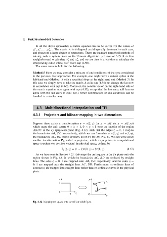
Suppose there exists a transformation r = r(ξ, η) (or x = x(ξ, η), y = y(ξ, η))
which maps the unit square 0 <ξ < 1, 0 <η < 1 onto the interior of the region
ABDC in the xy (physical) plane (Fig. 4.12), such that the edges ξ = 0, 1 map to
the boundaries AB, CD, respectively, which we can formulate as r(0,η) and r(1,η),
the boundaries AC, BD being similarly given by r(ξ, 0), r(ξ, 1). We can write down
another transformation P ξ , called a projector, which maps points in computational
space to points (or position vectors) in physical space, defined by

P ξ (ξ, η) = (1 − ξ)r(0,η) + ξr(1,η). (4.67)
As we have seen in Section 4.2.1 this maps the unit square in the ξη plane onto the
region shown in Fig. 4.8, in which the boundaries AC, BD are replaced by straight
lines. The sides ξ = 0, 1 are mapped onto AB, CD respectively, and the sides η =
0, 1 are mapped onto the straight lines AC, BD. Furthermore, co-ordinate lines of
constant η are mapped into straight lines rather than co-ordinate curves in the physical
plane.

h y
1 B D
C
0 A
1 x O
x
Fig. 4.12 Mapping unit square onto curved four-sided figure.