Page 101 - Basic Structured Grid Generation

90 Basic Structured Grid Generation

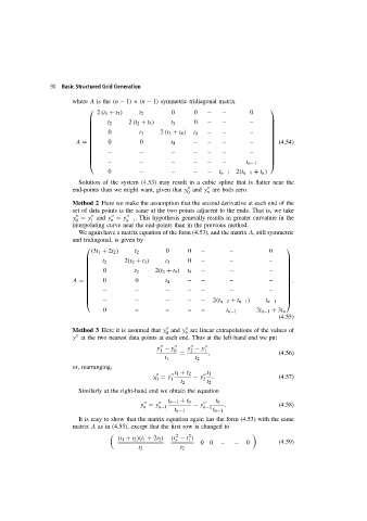
where A is the (n − 1) × (n − 1) symmetric tridiagonal matrix
2 (t 1 + t 2 ) t 2 0 0 – – 0
 
 2 (t 2 + t 3 ) 0 – – – 
t 2 t 3
 
 
0 2 (t 3 + t 4 ) – – –
 t 3 t 4 
 
0 0 t 4 – – – –  (4.54)
 
A = 
 
 – – – – – – – 
 
 
– – – – – – t n−1
 
0 – – – – t n−1 2(t n−1 + t n )
Solution of the system (4.53) may result in a cubic spline that is flatter near the

end-points than we might want, given that y and y are both zero.
0 n
Method 2 Here we make the assumption that the second derivative at each end of the
set of data points is the same at the two points adjacent to the ends. That is, we take

y = y and y = y . This hypothesis generally results in greater curvature in the
0 1 n n−1
interpolating curve near the end-points than in the previous method.
We again have a matrix equation of the form (4.53), and the matrix A, still symmetric
and tridiagonal, is given by
(3t 1 + 2t 2 ) t 2 0 0 – – 0
 
 2(t 2 + t 3 ) 0 – – – 
t 2 t 3
 
 
0 2(t 3 + t 4 ) – – –
 t 2 t 4 
 
0 0 t 4 – – – –  .
 
A = 
 
 − – – – – – – 
 
 
− – – – – 2(t n−2 + t n−1 ) t n−1
 
0 – – – – t n−1 2t n−1 + 3t n
(4.55)

Method 3 Here it is assumed that y and y are linear extrapolations of the values of

0 n
y at the two nearest data points at each end. Thus at the left-hand end we put

y − y y − y

1 0 2 1
= , (4.56)
t 1 t 2
or, rearranging,
t
t

y = y 1 1 + t 2 − y 1 . (4.57)
2
0
t 2 t 2
Similarly at the right-hand end we obtain the equation
t n−1 + t n t n

y = y n−1 − y n−2 . (4.58)
n
t n−1 t n−1
It is easy to show that the matrix equation again has the form (4.53) with the same
matrix A as in (4.55), except that the first row is changed to
2 2
(t 1 + t 2 )(t 1 + 2t 2 ) (t − t )
s
1
00 – – 0 (4.59)
t 2 t 2