Page 98 - Basic Structured Grid Generation

Structured grid generation – algebraic methods 87

We also have, in the obvious notation, r AB = r(0,η j ), r CD = r(1,η j ), r =
AB

r (0,η j ), r = r (1,η j ).

CD
4.2.3 Cubic splines

Fitting a single polynomial to a set of data points (x 0 ,y 0 ), (x 1 ,y 1 ), ... ,(x n ,y n ) is often
unsatisfactory, even for relatively low values of n, due to the fact that a polynomial
of degree N can have (N − 1) relative maxima and minima, so that the interpolating
curve may oscillate, or wiggle, excessively between data points and hence may not
appear to be a good fit. This difficulty may be overcome by generating a ‘composite’
interpolation curve, constructed out of low-degree polynomials fitted together in a
piecewise manner. Such curves are called splines. So when in a process of algebraic
grid generation we want to control grid distribution by prescribing a large number of
interior points, splines may be used as blending functions.
There are many ways in which piecewise interpolation may be carried out. Here
we concentrate on one of the commonest methods, that of cubic splines. In a cubic
spline fit the interpolating function between any two adjacent points is a third-degree
polynomial. For the (n + 1) data points above there are n intervals between the points,
in each of which a cubic polynomial is required. We can write these as
2 3
φ i (x) = a i + b i x + c i x + d i x for x i−1 x x i , i = 1, 2,...,n, (4.39)
for some constants a i , b i , c i , d i , to be found. Differentiation gives
2

φ (x) = b i + 2c i x + 3d i x ,
i

φ (x) = 2c i + 6d i x. (4.40)
i
We denote the overall piecewise-cubic interpolating function by y(x); the smoothness
of this function is made possible by arranging that its first and second derivatives are
continuous at the interior points x 1 ,x 2 ,...,x n−1 . So, in addition to the basic continuity
requirements
y(x i ) = φ i+1 (x i ) = y i , i = 0, 1,...,(n − 1),
y(x i ) = φ i (x i ) = y i , i = 1, 2,... ,n, (4.41)
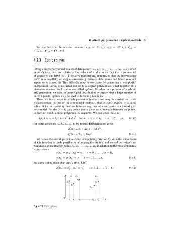
the cubic spline must also satisfy (Fig. 4.10)

φ (x i ) = φ (x i ) = y , i = 1, 2,...,(n − 1) (4.42)
i i+1 i
y f 1 f 2 f n
y 2
y 0 y n
y 1
y n−1

0
x 0 x 1 x 2 x n−1 x n x
Fig. 4.10 Cubic splines.